James K. Roberge: 6.302 Lecture 12
JAMES K. ROBERGE: Hi. To this point in the series, we've been concentrating on the analysis and design of linear feedback systems. As I'm sure you appreciate, the assumption of linearity is unrealistic for physical systems. Virtually any actual system is non-linear, to a certain extent, at least, when examined in sufficiently fine detail. Today, I'd like to start looking at techniques that allow us to investigate the behavior of non-linear systems. And we will continue this for the next three lectures.
As you appreciate from previous experience, non-linearities greatly complicate the analysis of any system. The familiar analytic techniques that we're used to using, particularly those based on frequency domain representations, are no longer directly applicable when we have non-linearities. And in particular, the difficulty comes when we mix non-linearities with dynamics.
We did early in the sequence look at an example of a nonlinear system, if you recall the audio amplifier that included a non-linearity. But there, we assumed that the system was dynamicless. There was no energy storage associated with the system. And there we found it was fairly simple to trace signal behavior through the system.
However, when we combine non-linearities with dynamics, we find that we have considerably greater analytic difficulty. I think we can emphasize that by considering that virtually anyone can learn to solve linear differential equations. And in fact, once you learn a few techniques for the solution of linear differential equations, why, you can basically solve any order linear differential equation. However, the few non-linear differential equations that we know how to solve exactly are in fact named for their solvers.
Today, I'd like to look at one particular technique for the analysis of nonlinear systems. It's not a general one. But it applies to an important class of systems. And that technique is linearization.
I think we've all seen this before in one way or another since it's a familiar tool to many engineers. For example, the relationship between the collector current of a transistor and its base-to-emitter voltage is highly non-linear. Similarly, the various junction capacitances of a transistor are again non-linear. They're dependent on operating point.
And yet we are able to make a linear model for a bipolar transistor and use that to predict the behavior of such a transistor in a variety of circuits. And that technique is of course one of linearization. And we'll expand on that idea today.
I'd like to remind you of the notation, since we will use it extensively in this session. In particular, the notation that we've been using throughout the subject is one that identifies the nature of a variable by a combination of the case used for the variable itself and for its subscript. And here, we see the four possibilities drawn out.
We have a total variable, which consists of a lowercase variable with a capital subscript. So we might have lowercase v sub cap O to indicate an output voltage, lowercase v sub cap I1 to indicate a first input voltage. So that's the total variable indication.
If we can decompose a total variable into the sum of an operating point and an incremental component, we designate the operating point or the bias value of the variable with a capital variable and a capital subscript. So again, we have capital V sub capital O for the operating point associated with an output voltage, capital V sub capital I1 for the operating point associated with one of the input variables. We use lowercase for both the variable and the subscript to denote incremental variables, as shown.
And the fourth permutation, which combines a capital variable with a lowercase subscript, indicates a frequency domain representation, either a complex amplitude or the Laplace transform of a variable or something like that. So that permutation, we use to designate a frequency domain representation.
Let's consider that we have an output defined as some general function of a number of inputs. And what we'd like to do is see how we develop a linear model that we can use to describe this relationship. The hope is that when we linearize our equation, we're at least able to predict the behavior of a system using that linearized approximation over some restricted range of variation about an operating point.
So our assumption is that we can, at least for some sufficiently restricted range of input and output variables, describe the total output, lowercase v sub cap O, as the sum of an operating point component plus an incremental component. And what we do in order to complete this expansion is to do a Taylor series expansion of the output about the operating point. And as you recall, in order to do that, we evaluate s the function at the operating point defined by the various input variables.
So we express the output as the sum of first of all, the function defined at the operating point. Then we take the derivative of the output with respect to the first input, evaluate that derivative at the operating point, and multiply this coefficient, which is now simply a number. Multiply this coefficient by the incremental change in the first input variable.
And we continue that expansion for all of the input variables. We take the derivative of the output with respect to the second input variable, evaluate that once again at the operating point, at cap VO or at cap VI1, VI2, and so forth. We evaluate this partial derivative at the operating point, multiply the resulting number by the incremental change in the second input variable, and so on.
Finally, we get to the derivative of the output with respect to the nth input variable, evaluating once again at the operating point and then multiply that coefficient by the incremental change in the nth input variable. And now, if we continued a Taylor series expansion, there would be higher-order terms associated with this collection. But all of those higher-order terms would involve products of incremental variables such that we have at least the square of an incremental variable or the product of one incremental variable times another one as the quantity multiplying our coefficient.
And if we restrict ourselves to sufficiently small variations in input variable, we argue that the second-order terms and higher terms can be neglected. And we can then base our approximation, argue that the incremental change in the output voltage is simply given by the various first-order partial derivatives multiplied by incremental changes in the various inputs. So we can use that truncated Taylor series expansion to develop a linear set of equations that describe our input to output relationship.
As an example of this kind of analysis, I'd like to consider the design of a system, which I think many of us have thought about. I know I spent an inordinate amount of time when I was a child worrying about this sort of thing. I didn't know then that it wasn't possible to do. And the problem is to try to suspend a magnetic ball, an iron ball, in a magnetic field. And I know, as I say, I spent an inordinate amount of time trying to figure out an arrangement of magnets that would allow me to suspend the ball in a magnetic field.
Well, it turns out that that's not possible. In fact, the general demonstration that it's not possible is known as Earnshaw's theorem. And the problem is that while we can find some point where the magnetic force exactly balances the force of gravity, that's an unstable equilibrium point.
If the ball gets a little bit closer to the magnet, why, the magnetic force increases. Of course, the force of gravity is constant. And so the ball is pulled into the magnet.
Consequently, if we move a little bit further away from the equilibrium point, why, the force from the magnet decreases. The ball falls further away. So we're not able to keep the ball fixed in a time-invariant magnetic field.
But there's a way to win this game. And in fact, it's used in, for example, the suspension of aircraft models in the MIT wind tunnel. What one does is build a system where you control the strength of the magnetic field. You measure ball position and then adjust the strength of the magnetic field in order to keep the ball a prescribed distance from the magnet.
And this system in front of me does this. Here, we have the base of it is simply a power supply. There's a large electromagnet that you can see.
There's a sensor, which is optical. And it consists of a lamp here with a little bit of a shield, very primitive optics, just a piece of cardboard wrapped around the lamp. Over in here, there's a photo cell, actually a photoresistor, that has a linear element, a linear sensitive area that's oh, possibly a quarter or 3/8 of an inch long. And again, extremely primitive optics, simply a washer in front of the thing.
The ball, then, casts a shadow on this linear photoresistor. And that gives us a method for measuring the position of the ball. And there's some electronics inside the chassis which drives a power amplifier, or a power transistor, on this heat sink. The output from the power transistor, the collector current of the power transistor, actually drives the electromagnet.
And the strategy, of course, is to measure ball position. When we notice that the ball has dropped further down, is falling away from the magnet, why, the system reacts so as to increase the magnetic strength. Conversely, as the ball moves up, why, the system works to decrease the strength of the electromagnet.
And if we do all of that correctly-- whoops-- we find out that the system will, in fact, support the ball in the magnetic field. We can maybe spin it. We can do a lot of things with the ball once it's in there.
As I say, this is used as a method for suspending aircraft models in MIT'S wind tunnel. It gives a very nice low-friction support so the forces of the support member don't influence the behavior of the aircraft model. Let's see how we make this go. Let's say it's a rather good example of linearized analysis.
Here we show very diagrammatically the system that we're using. We have an iron ball of mass m. And let's define the distance of that ball from some reference point as x sub B. If we were considering total variables, we'd a lowercase x sub capital B. And we observe the position of the ball, actually not with an eye, but rather with the photo cell lamp combination that I described a moment ago, and measure that way, get a signal proportional to the ball position, proportional to x sub B.
We take that electrical signal and amplify it. And as we'll see, we have to condition it as well. And that amplified measure of position generates a current, which we then use to drive the electromagnet. And as I described earlier, the strategy, of course, is as the ball moves down, we increase the strength of the magnet to pull the ball back toward its equilibrium position.
It can be shown that for certain choices of reference position, we can describe the relationship between the magnetic force in the upward direction on the ball and the two variables of interest, the magnet current and the ball position, as follows. The magnetic force on the ball is some constant, that depends on system geometry and parameters, times the square of the magnet current, divided by the square of the ball position. And we notice, of course, this equation matches the sort of observed behavior.
If we held magnetic-- the current constant as we, for example, increased the distance of the ball downward, we decrease the magnetic force. Similarly, as the ball moved upward, decreasing x sub B, we'd increase the magnetic force. And that's the observed behavior that makes it impossible for us to stabilize the ball in a fixed magnetic field.
Well, progressing as we had before, we can expand the magnetic force into the sum of an operating point component and an incremental component. So what we want to do is break our magnetic force into the sum of an operating point component plus an incremental component. And to do that, we first of all evaluate our expression for magnetic force at the operating point.
In other words, we have a term that's C times capital I sub capital M, the operating point value of the magnet current, squared, divided by the operating point value of the ball position squared. That's the value of the magnetic force, the operating point value, found by substituting in the operating point values for magnet current and ball position. So that's really this term.
Then we have the derivative of the original expression with respect to I sub M multiplied by the incremental change in I sub M. So the derivative of this expression is 2 C I sub M over X sub B squared. Again, of course evaluated at the operating point, capital I sub capital M and capital X sub capital B, multiplied by the incremental change in magnet current minus the derivative of our original expression with respect to x sub B.
And so when we do that, we get a minus 2I sub M squared over x sub B cubed times C, the coefficient shown, times the incremental change in ball position plus, of course, the higher order terms. And our hope is that, again, over some sufficiently restricted range of operation, we're able to ignore the higher order terms.
Well, let's use this incremental relationship between magnetic force and the two variables of interest, in particular magnet current and ball position, to write F equals m a, or, as I have things ordered, m a equals F. And that's simply the mass of the ball times the second derivative of ball position with respect to time, that's m a, equals the total force on the ball.
Well, m g, the mass of the ball times the acceleration of gravity, acts in a direction to increase x sub B. It accelerates the ball downward. So that comes in with a plus sign. That's the force due to gravity.
And the electrical force, or the magnetic force, acts to restore the ball. So we get the negative of the term shown above. So we get a minus CIm squared over XB squared minus 2CIm over XB squared times the incremental change in magnet current plus 2CIm squared over XB cubed times the incremental change in ball position.
Now we of course assume that the system is set up such that at the operating point, the operating point value of the magnetic force exactly cancels gravity. In other words, at the operating point, these two terms are equal and cancel. And then we're left with simply a relationship between the second derivative of ball position and the force that results from incremental changes in magnet current and incremental changes in ball position.
We can rearrange the equation in a somewhat more convenient form simply by multiplying through by the reciprocal of this term. And when we do that, we get the equation shown. mXB cubed over 2CIm squared-- that's the reciprocal of this coefficient-- times the second derivative of x sub B, with respect to t squared.
Also notice that the derivative of a total variable is identically equal to the derivative of the incremental component. The operating point, by definition, is a fixed quantity. And so when we take the derivative, why, that drops out. So we get m times the reciprocal of the coefficient shown times the second derivative of the incremental component of ball position with respect to time.
Again, when we do the multiplication, we get a coefficient here that's minus operating point value of ball position divided by the operating point value of the current times incremental changes in current, and then finally, plus the incremental changes in ball position. We can then transform that equation, recognize that the second derivative corresponds to multiplication by s. And things are further simplified if we just call this collection of constants 1 over k squared to save a little bit of writing.
If we combine those operations, that simplification as well as the derivative and transforming, we end up with an expression, s squared over k squared times X sub b, now of s, capital X sub lowercase b, the Laplace transform of the ball position, or the incremental component of the ball position, is equal to minus X sub B over I sub m times the transform of incremental changes in magnet current plus, again, X sub b of s. And in spite, of my attempt to be very, very careful with this, this should be a lowercase b.
We can rearrange that equation. Simply solve for X sub b of s. We get X sub b of s then being related to its second derivative multiplied by an appropriate coefficient plus X sub b over I sub m times I sub m of s.
And just to get a little bit of practice doing this, let's go ahead and make a block diagram for this particular equation. Let's see . We're going to solve for X sub b. And we notice that X sub b is related to two terms, or is a linear combination now of two terms. One is proportional to the magnet current, with a constant proportionality being Xb over Im, as well as a constant of proportionality times the second derivative of X sub b.
So as we construct our block diagram we're trying to solve for the variable X sub b. That variable is the sum of I sub m multiplied by a coefficient plus s squared over k squared, in other words, the second derivative, divided by k squared times X sub b. Those are the two terms that sum to give us X sub b.
So we get a little local loop in our block diagram that relates ball position to magnet current. This is the piece that we'd like to get. We will then make magnet current a function of ball position with an overall [? loop. ?] We can simplify this block diagram a little bit, collapse this loop. And when we do that, we get the forward path over 1 minus the loop transmission.
Well, the forward path is simply 1. The loop transmission in this case is plus s squared over k squared. And so we get an expression, the forward path, 1, over 1 minus the loop transmission, 1 minus s squared over k squared. And so this block represents or gives us the transfer function from here to here. We precede that with this block, and we get the overall relationship between ball position and the current in the magnet, or the incremental-- this equation, of course, or this block diagram relates incremental variables since we developed it via linearized analysis.
Again, we can rearrange terms just a little bit. It is a little bit more convenient probably to take the negative of the denominator, s squared over k squared minus 1, and counter that by taking the negative of the numerator. When we do all of that, we get minus Xb divided by Im. And we can then factor the denominator as s over k plus 1 times s over k minus 1. And so now we have a fairly convenient form for our block diagram that shows the relationship between ball position and magnet current.
We notice how the instability shows up here. When we look at the transfer function that relates ball position to magnet current, we notice that that transfer function has a pole in the right half plane. And we anticipate as a consequence of that that we get exponentially growing responses. And of course, that's what happens.
In a linearized analysis, if we looked at the behavior of the ball for small displacements from equilibrium, under the conditions of a fixed magnetic field, we'd find that as the ball sort of fell away from the equilibrium point, either fell downward acting under the force of gravity or fell upward into the magnet, the deviation from the equilibrium position would be exponential for small displacements, an exponentially growing displacement from the null position for small displacements. So that behavior is reflected by the pole in the right half plane in the transfer function that relates ball position to magnet current. Well, we can use that description of ball and magnet dynamics to generate a block diagram for our overall system.
So here, we have the block that describes the ball and magnet dynamics, the expression we had on the board earlier. We can consider the input to that block, of course, to be magnet current. The output is ball position.
And then what we do is complete our overall loop by taking an amplifier-- an amplifier with dynamics, presumably. We'll find out that we have to add some compensation. And so we take an amplifier with some dynamics.
And we operate on the signal, the electrical signal proportional to ball position with our amplifier. And the output of the amplifier is magnet current. So this then completes our overall loop. We complete the loop by surrounding the ball dynamics with our amplifier.
The dynamics of the magnet and ball system provide two poles. As we've mentioned earlier, one of these is in the right half plane. We have two poles at s equals k, and that's the one, of course, that gets us into trouble, the right half plane pole, as well as a pole at s equals minus k. Now we can look at that pole zero diagram, or that, in this case, pole diagram, and think a little bit about how we might stabilize such a system. I think the easiest way to determine the approach we should use to stabilizing the system is via root locus approach.
Let's see. If we first of all simply surrounded the ball magnet dynamics with a pure gain, in other words, if a in our overall system block diagram were frequency-independent, that doesn't work. Because as you remember, the root locus diagram for this sort of a system would simply be two branches which came together. They would meet at the arithmetic mean, which in this case, happens to be the imaginary axis, and then branch off along the imaginary axis. So as we increase the gain of our amplifier, a, what would happen is that one pole, the one that's giving us the difficulty, would move from its position in the right half plane, finally reach the imaginary axis.
However, as we further increased gain, we'd then get a complex conjugate pole pair on the imaginary axis. And the implication of this is that while we would have lost the exponentially growing response, we'd end up with an oscillator. This system, of course, once we have sufficient a to get the close loop poles out on the imaginary axis, describes an oscillator. And so that would be the situation where if we displaced the ball a little bit from its equilibrium position, it would simply vibrate with a frequency determined by how far out along this path we were, equivalently, how much a we had used.
In reality, there's problems with that. Of course, there are additional low-pass elements in the system. And so we wouldn't be able to even get to the pair of poles on the imaginary axis without having some dynamics associated with the amplifier.
The thing to do is add a zero. That oft-times works to help stabilize systems. Incidentally, it's worth pointing out here that this system, which has an open loop pole on the right half plane, in other words, the loop transmission includes a pole on the right half plane, is one that we can't use a very simple method for stabilizing.
We can't simply reduce a0, f0. There's an awful lot of systems where we can lower a0, f0. And while we may get a system with low desensitivity, it may not have very spectacular performance, at least that will stabilize the system.
Here, we don't have that out. If we start with a low value for a0, we just don't move this pole even to the imaginary axis. And again, while we can bring this pole left, why, it still remains in the right half plane. And so, this is a system where lowering loop transmission magnitude, which for many systems at least results in stable performance, fails.
Well, let's see. Suppose we add a zero. That's a good thing to do. And in fact, putting a zero anywhere in the left half plane improves the performance of the system.
For example, I could put a zero in here. We have to put it in the left half plane. But if I added a zero, for example, here, why, our root locus diagram would simply be such that this pole move toward the zero.
For sufficiently large values of a0, then, we'd get this branch in the left half plane. In the meantime, the branch starting at this pole would simply move left. So we could certainly, by adding a zero so at this point, for some range of values of a, have both closed loop holes in the left half plane.
Alternatively, we can add a zero maybe out here. And this is one of those systems where the trajectories circle around. So we'd end up possibly with a root locus diagram that looks something like this, eventually going in that way and out here.
And so once again, for sufficiently large values of a0, we'd have this branch in the left half plane. We'd have both of our closed loop poles lying on the left half of the s-plane. So adding a zero combined with a sufficiently large magnitude for a0 is certainly one way to stabilize this system.
The actual behavior of the system is a little bit more complex than this. There are additional poles beyond those associated with the dynamics of the ball magnet system. For example, the way the position detection is done is using a photoresistor. And that's a device that depends on optical carrier generation. There's a time constant associated with that process.
And so as the ball moves, the value of the photoresistor is not instantaneously proportional to ball position. There's a time constant associated with that, or at least to first order, we can model it as a single time constant. There is, incidentally, also a nonlinearity associated with that relationship. If one goes into details on the sensor that's used, the way the resistance of the sensor varies with ball position, and so forth, there's really a nonlinearity associated with that transfer relationship, the one that links ball position to the eventually generated electrical signal.
But again, if we did this analysis in detail, we'd linearize that relationship for sufficiently small perturbations from the operating point. The operating point here is chosen such that about half the photoresistor is shaded by the ball, shadowed by the ball. And again, if we did the analysis in great detail, why, we'd linearize the transfer relationship associated with that sensor. It would simply become another scale factor in our set of equations. But there is a time constant associated with it.
There may be additional time constants associated with the magnet. It's a fairly large magnet. There's several thousand turns. We may not be able to very rapidly change the current in the magnet. And so there's probably a time constant associated with the magnet.
If we use a lead network rather than simply a zero, we realize that adding a zero to the loop transmission implies somewhere, we have to have an amplifier that has unlimited high-frequency gain. That's probably not realistic. We probably have to have a pole associated with that zero. The normal lead network kind of transfer function, that would give us an additional pole. So there's certainly other poles in the loop transmission.
Suppose there were two additional poles. There's probably more than that, but let's consider this situation. You're not guaranteed anymore that you can stabilize the system.
There is a particular relationship, however, if these additional poles are sufficiently far from the origin. And one can go through that development. If they're far enough away, then the addition of a zero, appropriately located, makes it possible to stabilize the system.
And if we've satisfied that condition, let's see, the root locus diagram for this thing looks something as follows. There's one branch that starts here and moves to the right, goes to this zero. This branch goes outward. However, this is a more remote pole, and so initially, this pole closer to the origin has more influence on the behavior.
Since that branch is moving to the right, this is a system where the average distance rule holds. Since we have four poles and only one zero, the average distance of the poles corresponding to these branches must move somewhat to the left. So these two branches meet at a point somewhere in the left half plane.
And again, depending on the exact spacing involved, we might end up with a diagram possibly that did something like so, eventually, the branches going off, making angles of plus and minus 60 degrees, the third branch, of course, going off at minus 180 degrees. But if, in fact, the relationship between the zero location and the additional poles were correct or if these poles, basically, are sufficiently far out at sufficiently high frequencies, why then there's some range of a0 for which all the closed loop poles lie on the left half plane. In particular, once we've reached a value of a0 that gets this branch to this point, from that point on, until these two branches once again cross into the right half plane, we have a root locus diagram or a set of closed loop poles, that corresponds to stable behavior.
Well, I think it's important to look at the way one might really design a system like this. I think the important thing is to have an understanding of how the system works. And we've done that with the kind of analysis that I've shown on the blackboards.
And fine, that gives us a very good appreciation for the actual behavior of the system. We can, with the linearized analysis we've gone through, readily identify why the system should be unstable on an open-loop basis, if you will. The dynamics associated with the ball and the magnet have a pole in the right half plane. And we would certainly anticipate, then, unstable behavior unless we do something to counter that right half plane pole.
So we've seen that behavior. We've then used our root locus approach to give us a quick look at what we might do to improve the situation. And we've decided on a compensation strategy based on that. In particular, what we'd like to do is add a zero to the loop transmission. And hopefully, then, by combining the zero with an appropriate amount of a0, we're able to stabilize the system.
Well, we could on one hand, go ahead and make very precise measurements on the system, measure the mass of the ball, characterize the magnet, determine the constant c in the equation that relates magnetic force to magnet current and ball position and make a whole collection of very, very detailed system measurements. We could go in and precisely characterize the sensor. Again, as I had indicated, there's a nonlinearity associated with it.
And so we could somehow try to develop that relationship and linearize it and try to make an estimate of its time constant and include all that in our equations. I'm sure that we could take weeks at the analysis of such a system if we wished to. But there's probably a much more reasonable way to do it from an engineering point of view.
What I actually did when I put together this system was to go through an analysis very much like I've done here and convince myself that I sort of understood how things work. And then I went ahead and built the system and built it with provision to adjust the two critical parameters, in particular to adjust the gain of the amplifier, adjust the quantity a0, and also adjust the location of the zero. I had a reasonable guess as to what those quantities should be.
But certainly, when I first put the system together, as Murphy would have it, why, it was unstable. But at least I felt that those were the two variables that I'd have to adjust in order to improve the performance of the system. And I left provision for doing that.
And so what I did was adjust those variables, twist the pots, until finally, I managed to get the ball stable in the magnetic field. In fact, what we can do as an aid to that, and that was actually the process that I went through, is even when the system's unstable, before we have the zero location and the value of a0 in the proper range, we can reach into the field, into the active area, close to the null position, and we can effectively feel the behavior of the ball. And when we do that, there's two modes of behavior while the system's unstable.
One is just sort of the ball falls out of the field. It just either drops down when we let go of the ball, or it gets pulled up into the magnet. Well, that corresponds to the condition in our root locus diagram where we really don't have enough a0. In other words, that's the single exponential growth.
And what that tells us is that we haven't increased a0 sufficiently. We're still at the point where there's a pole associated with the system in the right half plane. We have a real exponential growth away from the equilibrium point. You can feel that. The ball just sort of tries to drop out of the field, or tries to pull up into the magnet as you let it go.
Another possibility is that as we hold the ball in the magnetic field and begin to loosen up on it a little bit, effectively, we provide additional damping to the system. As we begin to loosen up, why, the ball begins to vibrate, begins to jump. And that corresponds to the case where either we have too much a0, f0, so that we have closed loop poles out here because we have an oscillation, or we had the zero improperly located.
And if the zero were improperly located, these poles might never get into the left half plane. They might branch off the axis while they were still in the right half plane. And so that probably corresponds to the wrong location for the zero or too much a0. So we're able to use that kind of reasoning to guide us in the initial adjustment of a0 and the zero location. And by using that sort of reasoning, I was able to very rapidly get the system to stabilize, at least get the ball to support itself in the magnetic field.
Originally, it was very, very jumpy. And if you made any perturbations at all, why, the ball would fall out. But at least we could get it in the magnetic field. And once that happens, things are fine.
There are a couple of additional points on the box that I haven't used in this demonstration. One of these is a drive point. And what that allows me to do is inject another little current on top of the magnet current. There's just a connection basically via large resistor from the point labeled "drive" to the magnet current. And so we can then inject little incremental step changes in magnet current by applying a square wave to the drive terminal on the device.
At the same time, we can measure ball position. We have an output from the device that basically gives us a measure of ball position. It's an electrical signal proportional to ball position.
So what we're now able to do is measure the step response of the system. We can go ahead. The ball's in the magnetic field.
We can perturb it, perturb magnet current just a little bit. The loop should react. If we increase magnet current, the ball will move a little bit closer to the magnet.
As a consequence of that, the loop will react to lower magnet current to reestablish equilibrium. And we can observe the nature of that transient response. And it's the usual sort of wiggly second-order looking kind of transient response that we've seen in a number of other systems, once the system's stable.
Well, once we have that picture on an oscilloscope, we're very easily able to adjust the location of the zero and a0 to improve the nature of the transient response. And that becomes a very, very quick and easy adjustment to make. So once we've used this sort of analysis to understand the system and to find which situation we were in, which direction should we go in terms of zero location and a0 to at least get the system stable in an absolute sense, once we're to that point, we get it stable in an absolute sense, the rest of the sort of quote, "optimization," goes very, very quickly.
Because we can now look at a transient for the system. And we can see the effect on the transient of adjusting a0, of adjusting zero location, very rapidly improve the performance of the system that way. And that's exactly the way I did design the system.
To this day, I don't know the exact value of k, for example. I suspect it's somewhere on the order of 20 radians per second for this particular system. But I've never gone through that. I estimate that from really the location that the zero ended up with and the amount of a0 that I needed in order to stabilize things. So my guess is that the value k is somewhere on the order of 20 inverse seconds for this particular system.
There's an interesting variation on this theme that's used in another application. There's an application for a magnetic suspension system for energy storage. If you look at the numbers involved, it happens that you can store energy in a flywheel.
If you make the flywheel out of the appropriate materials, composites or something like that, you can store rotational energy in a flywheel. And the energy density is comparable to that of chemical fuels. You can, for a given mass of flywheel, get energy storage that's roughly comparable to the same mass of a fuel.
And this is a fairly popular way, or people are at least investigating this, for storage of electrical energy. You could somehow spin the wheel up using power derived from solar cells, for example, and then get the energy back out of the wheel at nighttime, when the sun wasn't shining. Or maybe use this as a method for an electric vehicle or to store energy for a vehicle.
One of the things you'd like to do in order to store energy efficiently is to have a frictionless support for the wheel. And so people have considered magnetic suspensions for that sort of system. There was a group at Lincoln Laboratory that was worrying about this. And they used a magnetic suspension system.
But again, you'd prefer not to have to spend a great deal of power in the magnet. You'd prefer not to have to use a large electromagnet, as I have, because the power to drive that electromagnet, of course, would have to come from somewhere. And you're trying to improve the overall efficiency of the system.
So what the people at Lincoln did was use a permanent magnet and put a winding on it. But now, there's a null position. You can adjust or select your operating point to be that where the force associated with a permanent magnet just balances the force of gravity. And when you do that, you still have to worry about the stability of the system.
So perturbations, you handle with a coil, in conjunction with the permanent magnet, that allows you to change the total magnetic field. You add the permanent magnet field to that associated with the coil. But operating points are chosen so that the magnetic field associated with the coil at the operating point is 0. And all the coil does is basically stabilize the system.
And you can put a little subsidiary loop around the thing with a rather long time constant, kind of adjusts operating clients to be the operating point where the coil current is 0. And that was the approach used. So that way, they effectively supported the spinning wheel in a magnetic field, in effectively a frictionless support, without having to put any power into the electromagnet. Yet they still retained the ability to modulate the magnetic field in order to stabilize the system. It's a rather interesting extension of this idea.
And again, we've seen that the ball, when started spinning, will continue for a very long period of time, again demonstrating the very nearly frictionless nature of the support provided by that sort of a magnetic suspension system. This has been just one example of linearized analysis. I mentioned to you that there are-- we've seen other examples, certainly the way we look at bipolar transistors, the way we analyze circuits involving bipolar transistors usually is by a linearized kind of analysis.
Next time, I'd like to look at another way of handling non-linear systems. And that one will be based more nearly on some of the frequency domain concepts that we've used for linear systems. It's called describing functions. And as I say, we'll look at that next time. Thank you.