James K. Roberge: 6.302 Lecture 18
[MUSIC PLAYING]
JAMES K. ROBERGE: Hi, much of our study of feedback systems has really revolved around trying to prevent oscillations in feedback systems. Or, even preventing getting very close to oscillation when we consider the relative stability of many of our systems.
Today, I'd like to look at the converse of that problem. In particular, let's consider what happens when we want to design an oscillator. And in fact, a good quality sinusoidal oscillator. An oscillator that provides very high purity sinusoidal signals.
As an example of describing function analysis, we had looked at one function generator loop, which combined a Schmitt trigger and an integrator. And we found out that that made a very convenient laboratory generator, in that we were able to get simultaneously square waves and triangle waves. And then by shaping the triangle wave, very frequently manufacturers use that technique to build an oscillator or a function generator that can also provide sinusoidal signals.
The problem is that it's very, very difficult to get sinusoidal signals with high spectral purity via that technique. You can get ones that have harmonic distortion, possibly as much as 50 or 60 dB below the fundamental. But it's hard to get anything better than that by shaping a triangle wave.
The typically very high purity oscillators use other techniques, and are really attempts to make a system that looks very much like a linear feedback system with a complex conjugate pair of poles on the imaginary axis.
One of the popular topologies is the Wien-Bridge oscillator. And I show that here. There is the bridge network that, at least in this implementation, consists of a series and a parallel branch using equal RC values.
And then again, in this implementation, we have an operational amplifier. And one way to view this thing is that the operational amplifier takes the output of the Wien-Bridge. And notice the amplifier is connected for a non-inverting gain of plus 3. We have the feedback resistor of 2 R1, an input resistor equal to R1. So from here to here, we get a gain of 3 plus 3 through the operational amplifier. And so what we have is an operational amplifier connected for a gain of plus 3, and then the Wien-Bridge taking the output of the operational amplifier and feeding it back into the positive input terminal of the operational amplifier. This is actually a positive feedback system as we'll see in a moment.
We can write the transfer function for the Wien-Bridge, itself. This is Vo as shown in the view graph where Vo is the output of the operational amplifier.
If we assume that the input impedance to the operational amplifier is sufficiently high so that the Wien-Bridge is not loaded by the input to the operational amplifier, then Va, which is the voltage coming out of the Wien-Bridge-- in fact, the voltage applied to the non-inverting input terminal of the operational amplifier, that transfer function through the Wien-Bridge is simply equal to RCS over R squared C squared S squared plus 3 RCS plus 1.
If we look at this transfer function, we find out that at low frequencies the phase shift approaches plus 90 degrees. At low frequencies, the S-terms and the S squared term in the denominator are small compared to 1. The numerator simply gives us plus 90 degrees of phase shift.
At sufficiently high frequencies, the S squared term dominates the denominator. We get something falling off as 1 over RCS at sufficiently high frequencies. And so we get minus 90 degrees of phase shift.
At the tuned frequency of the Wien-Bridge-- in other words, at S equals j omega, where omega is 1 over RC, the S squared term cancels the plus 1 in the denominator. At that point, the transfer function gives us a gain of RCS over 3RCS, or 1/3. So the Wien-Bridge then gives us positive phase shift at low frequencies, negative phase shift at high frequencies. And at a frequency omega equals 1 over RC, the Wien-Bridge gives us no phase shift. And an amplitude, or a magnitude, of 1/3 from the input of the Wien-Bridge to its output.
Consequently, if we around the Wien-Bridge with an amplifier with a gain of precisely 3, we can form a positive feedback loop where the loop transmission magnitude is precisely 1 at only one frequency. In particular, at omega equals 1 over RC. At that frequency, the Wien-Bridge provides an attenuation of 1/3. The operational amplifier, as I showed in the view graph, provides a gain of 1/3. Or I'm sorry, a gain of 3. And so we have a loop transmission whose magnitude is precisely plus 1.
We can see the effect of this by drawing a root locus diagram. Let me stress the fact that this is a positive feedback system. I've also normalized things to RC equals 1 second.
If we factor the denominator of the Wien-Bridge transfer function, of course, all the frequency dependent elements are concentrated in the Wien-Bridge. I've assumed the operational amplifier has negligible dynamics. We find that by factoring that denominator, we get poles at s equals minus 1.5 plus radical 5 over 2 minus 1.5 minus radical 5 over 2 for the two poles associated with the Wien-Bridge transfer function. And there is, of course, a zero at the origin reflecting the numerator.
Now, we normally have drawn root locus diagrams for negative feedback systems. But there's certainly no reason that we can't extend the technique to use it for positive feedback systems. And let's see what modifications we have to make to our rules.
We developed most of our root locus rules by arguing that in order to be at a point on the root locus, when we evaluated the angle of the af product that angle had to be an odd multiple of 180 degrees. In other words, the real part of the af product had to be minus 1. Or the real part had to be negative with no imaginary part in order to be at a point on the root locus diagram. That was necessary to cancel the inversion that in our standard topology, we assume occurs at the summing point.
If we don't have that inversion, if we have a positive feedback system, why the difference is that the rules that evolve from that 180 degree condition, we have to modify those rules to say that the angle associated with the af product now has to be a multiple, an integral multiple, of 360 degrees.
Well, one of the results of that is that branches now lie on the real axis where there are an even number of loop-transmission poles and zeroes to the right. So in this case, we have branches on the real axis here where we have two poles-- one pole and one zero to the right. And let's see, they also exist on the entire positive real axis where we have no poles or zeroes to the right. Again, an even number. And again, we can make appropriate modifications to the other rules.
We find out that if we evaluate the root locus diagram for this positive feedback system, these two branches simply come together. They break off the axis. And if we keep track of that, there's a rule that tells us where the breakaway point occurs. In particular, factoring the characteristic equation, or the loop-transmission with respect to S and setting that equal to 0. We find out the breakaway occurs at S equals minus 1. There's a reentry point at s equals plus 1. We've seen enough of this sort of thing to realize that we'll get a circle. Something like so.
The crossover into the right-half plane, of course, occurs for our normalized system with RC equal to 1. This is a circle. Breakaway is at minus 1. Reentry is at plus 1. This is plus j and down here we have minus j.
If we evaluate the gain necessary to get a pair of poles right on the imaginary axis, that's the oscillator condition, of course. We want to use this thing as an oscillator and have it provide sinusoids that are constant in amplitude, why what we want is to have a complex conjugate pair of poles on the imaginary axis. We find out that the a0 f0 necessary in our positive feedback system to bring us to this point is simply 3. We had argued that before on physical grounds, recognizing that at the frequency where we get no phase shift through the Wien-Bridge network, we had an attenuation of 1/3 through the network. We make up for that by surrounding the network with an amplifier that provides a gain of 3.
Well, when we go to do this, we have to worry somehow about stabilizing the system, stabilizing the amplitude of the oscillation. If we simply build up our linear system, of course, we'd never get things precisely right. The poles would either be in the left-half plane or they'd be on the right-half plane. We would never be able to get them precisely on the imaginary axis. So we have to somehow take care of that fact.
And at least one possibility is to modify our amplifier a little bit. As shown, our amplifier provides a gain of plus 3. However, we could make the feedback resistor, for example, nonlinear. Such that for small signals we got a gain of 3, and for larger signals we got a somewhat reduced gain. In fact, we have to do a little bit better than that.
The problem is that component tolerances tell us that for any real physical Wien-Bridge network, we'll probably need a gain greater than 3 in the amplifier in order to ensure that the poles are in the right-half plane. Or actually, to get the poles on the imaginary axis. The extent to which the gain has to exceed 3 is a function of component tolerance.
If the values are precisely as shown, we need a gain of exactly 3 in the operational amplifier, closed-loop gain of exactly 3. However, any deviation from that symmetry means that we need to gain somewhat greater than 3. And so we can, as a function of the kinds of components we anticipate, determine how much larger than 3 the gain of the amplifier must be to ensure that we will always be able to get poles at least on the imaginary axis.
We might do that by making one resistor that determines the gain of the operational amplifier R1, and a second resistor equal to 2 R1 plus 3 times delta R1.
If we evaluate the closed-loop gain of the amplifier, we'll then find out that the gain from here to here is simply equal to 3 times 1 plus delta where delta is presumably a small number. So that's fine. We can choose delta sufficiently large, so that we guarantee under small signal conditions that the poles of the system are in the right-half plane. Consequently, when we start the system up, we'll get an exponentially growing oscillation at approximately the desired frequency 1 over RC radians per second.
However, we have to do something now to limit the amplitude of the oscillation. And so now we could view the operational amplifier in a describing function sense. Let's design a system that has a gain for small signals that's 3 times 1 plus delta. But then let's put some sort of a limiter, possibly across this resistor. I've shown it again as a pair of back to back zener diodes. We saw in the last session that that was an effective way of providing a limiter.
In this case, in the non-inverting amplifier configuration, when signals become large enough to short out these diodes, the incremental gain from this point to this point does not go to 0. But rather, to unity. Because we have then, effectively a direct incremental connection between the output and this point. We have the non-inverting follower, the gain of one amplifier.
So if we plot the Va versus V out transfer characteristics, or V out as a function of Va, the slope will be 1 plus delta until we get up to a voltage equal to the breakdown voltage of the zener diodes. Beyond that, the slope is 1.
We can look at the describing function for that element. It starts out, of course, with the value of 3 times 1 plus a. When the test signal into our nonlinear element-- in particular, the amplitude of the signal here-- becomes equal to the zener breakdown voltage, the describing function magnitude begins to drop off. It eventually asymptotically approaches 1. And of course, we'd anticipate that our system would oscillate, assuming perfect components, symmetrical components, in the Wien-Bridge.
When the amplitude into our operational amplifier had become large enough, so that the gain of the amplifier from here to here in a describing function sense, lowered to 3. That's this point. So we'd anticipate that the amplitude of the fundamental component of the signal applied to the operational amplifier would be this value. That's the value that squeezes down the gain to precisely 3.
The difficulty with doing that is that we get harmonic distortion certainly. We would typically, in this situation, like to use the signal V out as the output voltage of our system because it's buffered. It comes from an operational amplifier. That'd be a nice point to use as an output for the overall oscillator. But that signal has harmonic distortion. And in fact, the harmonic distortion is unattenuated by the frequency selective network in this case. Because we apply the input to the amplifier here, the nonlinearity occurs in the amplifier. So it really squeezes down the top and bottom of the sine waves. We get some harmonic distortion out of that.
We can reduce the harmonic distortion by making delta small. In that case, we'd just sort of edge into the limiting characteristics of the zener diodes, get very little flattening, and very small harmonic distortion.
However, if we want to build a design that's relatively tolerant of inaccurate components, we have to make delta large enough to accommodate the spectrum or spread of anticipated component values. And again, if we are not awfully careful in our choice of components, delta may have to be fairly large to guarantee that every member of the population that we build up, if we build a bunch of these oscillators will, in fact, start oscillating.
We could, of course, tweak things up. But then there's temperature dependencies and that sort of thing that, again, lead us in the direction of having a conservative value for delta so that we're sure that all of the oscillators we build oscillate all of the time. And the effect of making delta larger, of course, is to increase harmonic distortion. Because for sort of a typical member of the population, we have to go very far out in the curve, get a measurable amount of flattening in the output sinusoid.
Another strategy would be something as follows. We could, for example, consider taking our oscillator and maybe have a potentiometer that allowed us to adjust gain. And we could look at the output of the amplifier, or the oscillator on an oscilloscope, for example. And if we found that the amplitude were shrinking, or were smaller than we wanted it to be, we might up the gain of the operational amplifier. That would, presumably, move the poles of the system either into or toward the right-half plane.
If we moved them into the right-half plane, the amplitude would begin to grow. We could let it grow to the amplitude we wished. And then, back off a little bit on the potentiometer. And hopefully, by us playing servomechanism, we could keep a constant amplitude oscillation. That, of course, is a little bit impractical. But it happens that some of the very high quality quote, linear oscillators, ones that give us very harmonically pure sorts of sinusoidal outputs, basically use this approach.
What they do is build up a feedback system that looks, in some sense, at the amplitude of the oscillation. And they then adjust some parameter in a loop on a very long time constant. They basically make a measurement over many, many cycles of oscillation and with a very long time constant adjust some parameter in the loop with the hope of keeping a pair of poles precisely on the imaginary axis.
I understand, although I haven't verified this myself. But I understand that one of the first products made by Hewlett Packard was an audio oscillator that basically used this technique. They used a Wien-Bridge kind of a circuit. As the variable element, they used an incandescent lamp. An incandescent lamp has temperature dependent resistance. And by applying the signal in the Wien-Bridge, the lamp formed part of the Wien-Bridge. As the signal got bigger or smaller, the resistance of the lamp changed because of heating in the lab. That occurred with a very long time constant, at least compared to the period of oscillation. And the resistance of the lamp changing would automatically act to stabilize the amplitude of the oscillation. It's kind of an interesting passive, if you will, feedback system.
I also understand, but I'm not sure how true that is, that that oscillator was originally developed for some early Walt Disney movies. But I haven't verified any of that personally.
What I'd like to do is look at an example of an oscillator that basically uses this technique. We won't use a Wien-Bridge. I'd like to introduce another topology for an oscillator.
And the oscillator that I'd like to look at is called a quadrature oscillator. And it consists of two integrators.
Here we have a familiar non-inverting integrator. Or, I'm sorry, inverting integrator simply R and C. So the transfer function from here to here is minus 1 over RCS.
The other configuration is a little less common. It consists of a low pass RC section. And if for a moment we assume that delta is equal to 0, we then have a CR from the output back to the inverting input of the operational amplifier.
And if you write the transfer function from here to here for delta equals 0, you find out that that transfer function is plus 1 over RCS.
So if delta is 0, if the RC's are matched, we have a minus 1 over RCS from here to here. We have a plus 1 over RCS from here to here. We have a system whose loop-transmission is minus 1 over RCS quantity squared. And it's quite easy to show that that gives us a pair of poles on the imaginary axis.
Again, we have the problem of stabilizing the amplitude of such an oscillator. Well, let's see. Let's consider what happens if we allow delta, as shown in the view graph, to be variable. Let's let that be our pop, the thing that we're going to adjust to control the amplitude of the oscillation.
We can write the loop-transmission, or maybe the negative of the loop-transmission as simply 1 over RCS. That's the transfer function of the first integrator. Or actually, the negative of it. The first integrator gives us an inversion. And we'll take the negative of that to get minus L of s. So we get 1 over RCS.
We then have the low pass characteristics of the RC that proceeds the second operational amplifier. We get 1 over RCS plus 1. And then we write the transfer function that links the output that gives us the gain from the non-inverting input terminal of the second operational amplifier to its output.
And if we write that exactly, we find out that that quantity is 1 plus delta R plus 1 over c over 1 plus delta times R.
If we collect terms, we find out that we get a 1 over 1 plus delta, a 1 over RCS quantity squared. And then we get a pole zero doublet. If delta is small, the doublet, of course, is closely spaced. A positive value of delta-- in other words, if the resistor going to ground is larger than the series resistors in the input RC network, then in fact the zero lies at a lower frequency than the pole.
We can analyze this system in a variety of ways. One fairly convenient way is to use a root locus approach. And if we draw a root locus diagram for the system, we find that we have a pair of poles at the origin associated with the loop-transmission. That's the one over RCS quantity squared. And as I have shown things, we have a pole at s equals minus 1 over RC here. We have a zero located at a slightly lower frequency, a slightly longer time constant. In fact, we have a zero that's at minus 1 over 1 plus delta times RC.
And if delta's small compared to 1, we can use a series expansion for 1 over 1 plus delta and approximate that series by its first term. And under those conditions, we get this at approximately minus 1 plus delta divided by RC. That's the location of the zero in the loop-transmission.
Well, the root locus diagram for this set up, of course, is simply that this branch moves toward the zero. To counter that, this is a system where the average distance remains a constant because we have three poles and only one zero. These branches spring out at right angles, o spring out along the imaginary axis. But they have to come back somewhat to counter the fact there's a branch moving to the right in the s-plane.
Asymptotically, for very large values of a0 f0 product, let's see. This moved to the right an amount delta. Each of these branches would have to move back an amount delta over 2. We can get that, as I say, either by the average distance argument, or by calculating asymptotes for these branches. In either case, we'll find out that they move back an amount delta over 2 times RC.
For the a0 f0 that corresponds to this expression, we find out that the closed-loop poles of the system lie here. And of course, the complex conjugate to that point. And they have an imaginary part equal to simply 1 over RC, or j over RC. And the displacement from the real axis, this quantity, is an amount delta divided by 4 RC. It's fairly easy to show that by directly factoring the characteristic equation that corresponds to this expression for the negative of the loop-transmission.
Well, now we see our strategy. As we change delta, we move the location of this zero. A positive value for delta gets us a situation shown, which results in a stable system. All the closed-loop poles lie in the left-half plane.
If we make delta negative, make the resistor going to ground smaller than the series resistor going into the operational amplifier, make that time constant a little bit shorter than the input time constant, then this zero's on the other side of the pole.
Under those conditions, the closed-loop poles are in the right-half of the s-plane. And so now our strategy parallels that that I suggested for the Wien-Bridge.
We can look at the amplitude of the oscillation being generated by our system, and we effectively have a pot that changes delta.
What we would do is increase delta, make delta positive if we found that the amplitude of our oscillation was too large. Because that would move the closed-loop poles to the left-half plane. The amplitude would begin to shrink. When it had shrunk back to the right size, we presumably would change delta such that the closed-loop poles lay exactly on the imaginary axis. And then, from there on in, keep adjusting the pot to make up for very small changes in system quantities in a consequence of temperature dependence, or aging, or whatever. And work to keep the output amplitude constant.
To the extent that we were able to keep these poles, closed-loop poles precisely on the imaginary axis by making this 0 lie precisely on this pole, we'd have a constant amplitude oscillation, which would be harmonically pure. We have a true linear system with a complex conjugate pair of poles on the imaginary axis. How might we physically accomplish that?
The possibilities are to use a field-effect transistor in order to vary the resistor. At least that's one possibility. We notice the resistor, whose value is 1 plus delta times R, associated with the right-hand operational amplifier. We could make part of that resistor, for example, be a field-effect transistor. And for small signals applied from the source to the drain of the field-effect transistor, why we're able to change its resistance. It behaves like a linear resistor. And we can modulate its value. And so that might be a mechanism for controlling amplitude.
What our strategy would be, would be to measure Va, determine the amplitude Va somehow. And then, build a control loop that changes delta in an attempt to keep V sub a constant.
One of the interesting fringe benefits of the use of a quadrature oscillator, which is of course, where it gets its name, is that when we have the loop running, we ideally have two integrators ganged up. And so we get two sinusoidal signals. We've been focusing only on Va in the discussion, but we do get two sinusoidal signals, which happen to be 90 degrees out of phase since they represent respectively the input and outputs of integrators. And that is a very useful feature in certain instrumentation applications.
Let's see how we really control the amplitude of this oscillator. I've mentioned the overall strategy, but now we have to think a little bit about how we model this system. And in particular, one of the variables is how does Va react, the signal amplitude, or actually the envelope of that oscillation react, as we change delta?
What we're really going to do here, you see, is build a very, very slow loop that controls the amplitude of the output signal. And there's sort of two independent feedback processes going on at once. One of them is the double integrator loop that crosses over at a fairly high frequency. At a frequency omega equals 1 over RC. And that's the basic oscillator. We're oscillating basically, at a frequency 1 over RC radians per second.
The other one is a much, much slower loop, a much lower crossover frequency that works on the amplitude of the signal. And so what we have to do works on the envelope of the signal, to keep that envelope constant in amplitude. So what we have to do is figure out a way to model the transfer function really that goes from changes in delta to changes in amplitude. Our feedback system is going to measure amplitude, feed back to control delta. And clearly, part of that loop, is the delta to envelope or amplitude transfer function. We have to find out how we model that or how we represent that.
Well, to do this, let's assume that our system is oscillating with the actual signal V sub a being equal to some E sub a, an amplitude associated with that signal, times sine omega t. And omega is equal to 1 over RC. This is the situation that results with perfectly matched components, delta equals 0. We have a pair of complex conjugate poles on the imaginary axis. We get a pure sinusoidal oscillator and the amplitude is a function of initial conditions.
Now, let's see what happens if we make a step change in delta. So we change the value of that resistor at time t equals 0 to some value delta 1. We put in a step at time t equals 0 of magnitude delta 1.
Well, for time greater than t equals 0 then, the voltage V sub a will be exponentially decaying. we found out that positive values of delta at least give us poles in the left-half plane. And so there may be a little bit of phase shift, a phase change, but that's not very important. We're going to focus principally on the envelope.
Our signal V sub a is then, again, E sub a. That was the value I had initially times sine omega t. Times E to the minus delta 1 t over 4 RC. Reflecting the fact that the poles have a real part that's minus delta over 4 RC. So we get the minus delta 1 over 4 RC times t as the exponent.
And we can look at this, we can look the actual envelope. Here we're going ahead. The oscillation is running along in here at a high frequency. In fact, determined by the RC constant. So this is running along like so. Prior to time t equals 0, delta is 0. So the amplitude of the oscillation is constant, and the magnitude is E sub a.
For times greater than 0, the amplitude decays exponentially. The envelope going as E sub a, E to the minus delta 1 over 4 RC times t. So we have the oscillation running back and forth. Constant amplitude up to time t equals 0. For a positive value of delta, an exponentially decaying amplitude thereafter.
Let's go ahead and write E sub a, the total variable associated with the envelope. Well, the envelope is our initial amplitude. The envelope amplitude E sub capital A times E to the minus delta 1 t over 4 RC. And what I'll do is expand that in a series, recognizing that the term, the exponential, is hopefully small. Delta is a very, very small quantity.
And if we do that, we get the first two terms of this series being equal to capital E sub capital A. That's the initial amplitude. That's this value. Minus delta 1 Ea over 4 RC times t. And then there's the quadratic term and all of that.
If, in fact, this quantity, the exponent is small enough, we can make a linearized approximation to this transfer, or to this behavior. And we'd recognize capital E sub capital A is the operating point value of the envelope. And then this term is the incremental component. So that's the usual linearized analysis where we consider only the first two terms in the series expansion. Or actually, the operating point value plus the first term in the series expansion for the envelope. Again, I emphasize the fact that our strategy is going to be to measure the envelope. Hopefully do that without regard for the actual oscillation. We'll try to build some sort of a detector that measures envelope, do that without worrying about the exact details of the oscillation, and then use envelope information, measured envelope amplitude to control delta. Well, fine.
What we find out is that we make a step change in delta. And the incremental component, when we draw an incremental block diagram or a linearized block diagram, in response to making a step change in delta, we get a negative ramp for the incremental change in the envelope. E sub a is something times t.
Well, let's see. We have a system that we are assuming is linear by virtue of the fact that we've performed a linearized kind of analysis. We're doing an operating point plus a linear change from that operating point sort of analysis. So we have a linear system. We put in a step and we get out a ramp. We conclude that the transfer function that relates output to input for such a system must be simply an integration. When you put a step into an integrator, you get a ramp out.
Consequently, the fourth permutation in our hierarchy of variable and subscript, E sub a of s, the transfer function that relates the transform of the incremental component of the envelope to delta, is simply the scale factor that we got from the earlier equation minus E sub cap A over 4 RC, now times s reflecting the integration associated with our linearized analysis. The fact that a step gives us a ramp change in envelope. That's simply saying that if things go for a short period of time, if we look at the system for a short period of time, there's a funny kind of linearization here. You're linearizing a variable that runs continuously. But what happens is that the system works to force itself back to equilibrium in such a way that this exponent stays pretty small. The total exponent stays pretty small. It goes to 0. The feedback system works in that direction.
Well, to the extent that we can use that sort of linearized analysis, we're able to model this thing as simply the integration. And now we can draw a block diagram.
We have a reference value for our envelope. We have the actual measured envelope amplitude. We compare those two. We go through some sort of a controller, and then we go through the dynamics that relate envelope to delta. So this point in the block diagram is really delta of s. We go through the transfer function we developed above, capital E sub capital A over 4 RCS. That gets us an output amplitude. We compare that with a reference amplitude modified as we need to with our compensator, or loop gain, or whatever, and that completes the loop.
Since there's a minus sign associated with this relationship, we'll find out that a of s actually has to be negative, itself so that we end up with a negative feedback system.
When we go to do this, there's some practical things that we have to consider. One is that in order to make our analysis valid where we sort of ignore the structure associated with the high frequency oscillation, the oscillator is going providing a high frequency oscillation. In order to ignore that structure, we have to have the crossover frequency in the loop that controls the amplitude of our oscillation much, much lower than 1 over RC. As we approach 1 over RC, we get into sampling kinds of problems. We're not able to get a good estimate of the envelope on an instantaneous basis.
And the thing that allows us to get a good estimate on a sort of instantaneous basis compared to the dynamics of our amplitude stabilization loop is to ensure that the crossover frequency in that loop is much, much less than 1 over RC.
We also might like to have a system that will force the output amplitude to be identically equal to the reference amplitude. And in general, that requires some voltage, for example, on the control, the gate of our field-effect transistor. And the way we can support a finite voltage with zero error is to simply use an integrator. And so let's design our a of s to include an integration. That will ensure, as I say, that we can get any voltage we need to control the loop with negligible error, zero error, between our commanded and actual value for the envelope.
Also, we need some filtering. If we think about the way we'll do this, we can't get a perfect detection of envelope. What we might do, for example, is a full wave rectifier. That's one possibility. Actually, the actual circuit that we'll look at is a little bit more sophisticated than that. It does some phase shifting, and then a rather neat multi-phase envelope detector that gets a fairly small ripple. It's equivalent to using several different phases. And just getting a scalloped kind of an output wave form. But there is still some harmonic content, some high frequency noise associated with that measure of the envelope. And what we have to do is filter that. Because if we think about the overall loop, we're going to apply some measure of the envelope or the error to our control element, to a field-effect transistor possibly if we use that as the control element.
And while I think the analysis is difficult, probably beyond my capability, modulating the control element at some high frequency can't possibly be good. We'd like to have the control element have a fixed value of resistance over an entire cycle, or many cycles of oscillation. So what we'd like to do is include a lot of filtering, so that this high frequency trash that's a consequence of our envelope detection gets filtered out to insignificant levels.
And finally, we have to be very conservative in our design. Because there's a lot of unknowns here. There's a linearity problem. Notice that the loop-transmission magnitude is a function of the commanded value for the operating point value for the envelope. So if we command a large envelope, we get a high loop-transmission. If we command a small envelope, we get a small loop-transmission. That sort of behavior, incidentally, is very, very, or always occurs in gain control kinds of things. You invariably find out that some loop-transmission parameter, some loop-transmission magnitude is dependent on operating point. It shows up here in our amplitude stabilization loop by virtue of the operating point value of the envelope coming in as a multiplicative factor in the loop-transmission.
There's a host of nonlinearities in the system. When you use a field-effect transistor as a control element-- and I do some of the analysis in the text-- we find that it has rather grossly nonlinear characteristics between control voltage, gate voltage, and incremental resistance when we use it in this mode. Really, our system loop-transmission magnitude at low frequencies may not be what we think it is. So we ought to design the system to be very, very conservative. Design a system that has plenty of phase margin under nominal conditions, so that when things are not as we thought they were, we still have adequate phase margin.
A possible a of s might be of the following form. We want an integration, so we get a0 over s. That gets us the integration. I will then go ahead and put in a zero. Because once we have the integration that we've intentionally added, we have that integration plus a second integration that occurs as a consequence of the dynamics that relate envelope to delta. And so what I'd like to do is add a zero, so that I get a 1 over s squared roll-off at low frequencies. Then a 1/s roll-off in the vicinity of crossover. Let's shoot for crossover at 10 to the minus second over RC, 1/100 of the frequency of oscillation.
I mentioned earlier we simply want to be at a small fraction of the frequency of oscillation. So let's assume we're going to cross over at 1/100 of 1 over RC. Let's put the zero a decade below that. That's quite conservative. We said with lag networks that we might start there, but then edge up. Let's put a zero, so we have a 1/s slope that extends from-- that starts a decade below nominal crossover.
And then I'll put two more poles that provide filtering a decade above nominal crossover. Again, recognizing that we're going to shoot for a crossover in the amplitude control loop that's 1/100 of 1 over RC. Let me put two poles that will provide additional filtering to signals at and above 1 over RC, the sort of hash on our envelope detector. Let's put a couple of filters that occur a decade below that. And in fact, are located one decade above our nominal crossover frequency.
We can adjust a0 then, so the crossover does in fact occur at 1/100 of 1 over RC. We'll have a loop-transmission that falls as 1 over omega squared at low frequencies. 1 over omega-- actually, for a decade either side of crossover if everything occurs as we hope. And then, as 1 over omega cubed beyond that.
If, in fact, our system were precisely like this, we would have about 75 degrees of phase margin. A very, very conservatively stable system. If this was the kind of a loop-transmission plot that we had.
Let's focus a little bit again on this relationship. The fact that we'd like to cross over at a frequency small compared to the oscillating frequency so that we don't get an interaction, a sampling kind of a thing. The only converse to that, normally you see our amplitude control loop only has to make up for aging, and temperature changes, and that sort of thing. And so a very slow amplitude loop is perfectly fine.
However, it's possible in some applications that we might want to make the command changes in the amplitude of the oscillator. And if we do that, then we'd like to have a reasonably high crossover frequency in the amplitude control loop, so that we get fairly fast response to commanded changes. I haven't tried to push that at all in the system we're going to demonstrate. What we'll do is really design for a nominal crossover frequency that's 1/100 of the oscillating frequency.
And here we have the experimental system that does this. There's a collection of operational amplifiers, and I won't go through all the details of that. But there are a number of operational amplifiers. The two basic ones doing our quadrature loop. There is another operational amplifier that really mechanizes a of s. And then there's several more that do the rather sophisticated envelope detection, a very low ripple type of envelope detector, multi-phase sort of envelope detector. So that's what the collection of operational amplifiers is used for.
There's a couple of switches. One which commands internally a fixed amplitude for the oscillation. And the other position of that switch allows us to externally command the amplitude, so we can, for example, look at the step response when we command a change in amplitude.
There's another switch that allows us to use external compensation. I won't do that in this case.
And we have, again, the power supply test generator that allows us to command changes in amplitude, and we observe everything on the oscilloscope.
What we're looking at here is the output without any commanded changes in amplitude. So we simply have a constant amplitude sinusoid. In this case, we selected the RC product to be 10 to the minus fourth seconds. We'd anticipate oscillation then at 10 to the fourth radians per second. We're at 200 microseconds per division. To again, within the ability of our measurement, we find out that we get an oscillating frequency that's sort of 10 to the fourth divided by 2 pi. A period of something over 600 microseconds, three divisions.
If you investigate this with a spectrum analyzer, you find out that this is a very, very pure sine wave. The sort of distortion we get verifies the basic design principle, the idea of using this as a technique for stabilizing the amplitude of the oscillator. The harmonics distortion in this one is 80 or more dB below the fundamental. So the idea of putting in a slow loop to control the amplitude does a very, very good job of reducing or of giving us a spectrally pure output.
What we're now able to do is change the switch that connects us from an internal reference for that amplitude-- the amplitude now is about 5 volts peak or 10 volts peak to peak-- to an externally commanded reference. And we'll put a square wave in as the command. So let's simply throw this to the other position.
Now we see the modulation. We're, again, modulating at about the same amplitude as we had before. Let's go to a situation now where we can look at the envelope, and let's trigger off the signal generator.
And now what we see is exponential, basically exponential changes in the envelope. Here we're commanding a smaller envelope. Here we're commanding a larger envelope. Let me just speed this up a little bit if we can. That's too fast.
Again, here we see the exponential changes. Commanding a small amplitude, then commanding a larger amplitude. Operating about 5 volts.
For this small a signal, things are relatively symmetrical. We could estimate crossover frequencies in the control loop by looking at the time constant of this exponential. Since we have a system with high phase margin, we design for 75 degrees of phase margin, we get responses that look very, very much first-order.
If we had 90 degrees of phase margin, we'd anticipate responses that are indistinguishable from first-order responses. This looks very, very much like a first-order exponential. And the time constant of the change in envelope is the order of 10 milliseconds, the 1/100 of 1 over RC that we shot for. Let's now look at what happens when we put in larger commanded changes. So I can do that. Let me lower the scale on the oscilloscope a little bit, and then just drive the system a little bit harder.
And now we begin to see how the nonlinearity shows up. There's a number of nonlinearities in the systems as I mentioned. Some of them have to do with nonlinearities associated with the control elements, the field-effect transistors, for example. There are other kinds of nonlinearities in the system. We mentioned also that the loop-transmission magnitude is dependent on actual operating condition. And when we put in large changes, our assumption of linearized analysis is not operation that's well-modeled. As incremental changes around an operating point becomes invalid, we're making now changes that are large compared to the operating point.
We find out that the way this manifests itself in this particular system, although there's no generality here, is a very non-symmetrical kind of change. The increasing amplitude, the dynamics associated with an increase in amplitude are much longer than the dynamics associated with a decrease in amplitude. But as I say, there's no real generality there. That's just a peculiarity of this system. Again, we can move up the overall amplitude. There we get into saturation.
But again, we notice here the fall time, if you will, the change to decrease smaller amplitude is considerably faster than the time necessary to increase the amplitude. So we see, at least, an indication of the nonlinearity associated with this system. Or some of the nonlinearities associated with this system.
In conclusion, I'd like to emphasize that this technique gives us the ability to build a very, very low distortion oscillator. And also, is a very interesting example of a feedback system that has two very distinct modes of operation. The basic loop that sets the frequency, the 10 to the fourth radians per second, or 1.6 kilohertz in this case. And then the much slower loop that controls the amplitude of that oscillation. And this sort of a system is an example of that's sort of interesting interplay between dynamics in a system that has two distinct modes of operation.
This concludes our discussion of oscillators. Thank you.