James K. Roberge: 6.302 Lecture 05

[MUSIC PLAYING]

JAMES K. ROBERGE: Hi. Today, I'd like to continue the discussion of root locus techniques that we started in the last session. As you recall, root locus is one of the two principal methods that we're going to use to evaluate the stability of feedback systems. The advantage of this technique, along with the second technique which we'll introduce later, is that it gives us a way to start with readily identifiable quantities, in particular, the loop transmission of the feedback system and, by rather straightforward analytic manipulations, determine the closed-loop transfer function or at least the important features of the closed-loop transfer function.

We also find out that, in addition to getting a binary answer to the stability problem, in other words, are there any poles of the closed-loop transfer function in the right-half of the s-plane, we're also able to get a very good analog measure of relative stability. In other words, we can find out how close our system to instability. We can tell, once we determine that our system is stable, what the damping ratio of the dominant closed-loop pole pair is. And in fact, we can determine many other features of a closed-loop response that we might be interested in.

If you recall, last time we in fact looked at a root locus diagram. Remember that we present the results of root locus analysis in a root locus diagram. And we started with a particularly simple system. In particular, we started with a system that had two poles associated with a loop transmission and no zeroes.

Both of those poles were located on the negative real axis at minus 1 over tau a and minus 1 over tau b. We then went ahead and wrote an expression for the closed-loop transfer function and focused our attention on the characteristic equation, in particular, the denominator of the closed-loop transfer function, we were then able to solve that characteristic equation, solve for the roots of that characteristic equation, by setting it equal to zero. And since the roots of the characteristic equation are the poles of the system closed-loop transfer function, we could determine how the closed-loop transfer function poles varied, in particular, as we changed A-naught, F-naught for the system. Recall that A-naught, F-naught is the magnitude of the low-frequency loop transmission of the system.

When we performed that calculation, again, by directly factoring the characteristic equation, we found that the closed-loop poles start very close to the location of the loop transmission poles for small values of A-naught, F-naught in this particular system. And then, as A-naught, F-naught increases, the two closed-loop poles move closer together and finally become coincident on the negative real axis at a location that's actually the arithmetic mean of the two loop transmission pole locations. Further increases in A-naught, F-naught beyond that necessary to get the two poles coincident, result in the two poles branching off the real axis and getting an increasingly large imaginary portion.

As the two closed-loop poles become a complex conjugate pair with an increasingly large imaginary component, the real part stays fixed. And so, as A-naught, F-naught increases, why the two complex conjugate poles move off north and south in the s-plane. Of course, they have to be symmetrical with respect to the real axis, since this corresponds to the pole locations for a physically realizable system.

We found that we were able to determine the closed-loop pole locations for our second-order system by directly factoring the characteristic equation. Unfortunately, that operation becomes tedious for anything other than first- and second-order systems. And so, today, we'd like to look at the way we can construct a root locus diagram without having to directly factor the characteristic equation.

Recall, we have a standard topology which has a forward path transmission, a of s, and a feedback path transmission, f of s. When we write a closed-loop transfer function for the system, we, of course, find out that capital A of s, the input to output transfer function, is simply equal to the forward path transmission over 1 minus the loop transmission. We're not particularly worried, initially, about the location of zeroes. Our initial consideration is with root locus techniques.

We'll focus only on how we find the poles of the system. Consequently, we'll look only at the characteristic equation, which we recall is 1 minus the loop transmission. That characteristic equation is, of course, common for any system with equal values for the af product. Remember that the zeroes of a closed-loop transfer function are dependent on how dynamics are distributed between the forward path and the feedback path. But the poles of a closed-loop transfer function are dependent only on the af product.

Well, when we calculate the characteristic equation, or 1 minus the loop transmission, it's simply 1 plus a of s, f of s, recalling that the loop transmission is minus a of s, f of s. Then we conclude that the poles of the closed-loop transfer function, capital A of s, occur when one plus of a of s, f of s equals zero. We may choose to express the af product as being equal to A-naught, F-naught times some g of s, where we've included all of the frequency-dependent portions of the loop transmission in g of s.

And furthermore, we'll choose to write g of s in a form such that g of zero is equal to 1. We'll normalize g of s so that the dc value of g of g of s is 1. In that case, the quantity A-naught, F-naught has the physical interpretation of being the magnitude of the dc loop transmission.

Suppose we'd like to perform a test. Suppose we're told that a particular system has a closed-loop pole at a point in the s-plane, S1, and we'd like to check to see if that's really true. Well that's easy to do.

If we're at a closed-loop pole, the characteristic equation, the denominator of any transfer function for the system, must, in fact, be equal to zero. That's what we mean by a pole. The denominator goes to zero. Consequently, the transfer function in question becomes infinite.

So if we are, in fact, at a pole of capital A of s, the quantity 1 plus A-naught, F-naught times g of s1 must be equal to zero. We can rearrange and recognize that that tells us that A-naught, F-naught times g of s1 must be equal to minus 1. Since A-naught, F-naught g of s, in general, is a complex number, we have to satisfy two conditions simultaneously to make it equal to minus 1. In particular, the magnitude of A-naught, F-naught times g of s evaluated at the point s equals s1 must be equal to 1.

And simultaneously, the angle of the transfer function A-naught, F-naught g of s evaluated at the point s1 has to be equal to an odd multiple of 180 degrees. However, since we've chosen to include all of the dynamics of our loop transmission in the quantity g of s, the angle condition reduces to simply having the angle of g of s1 being equal to an odd multiple of 180 degrees. What we recognize in this expression, n as an integer.

Just to refresh your memory, recall that, if we go into the s-plane and want to evaluate a function of s at some point in the s-plane-- suppose this is the point of interest, s1 and we're trying to check and see if that point, s1, in fact, satisfies the conditions for being a pole of capital A of s-- we can do the following. We draw vectors from the poles and zeroes of the af product, or the g product, to the point in question.

Here we have shown one real axis pole of g of s, a two-complex conjugate or complex conjugate pole pair of g of s and a single zero of g of s. If we now try to evaluate g of s at the point s1, what we do is draw vectors from the poles and the zeroes of g of s to the point s1. And I've showed that for the three poles and for the zero.

And we can evaluate the angle and the magnitude associated with those vectors. In particular, let's call this angle theta 1 and, similarly, the length of this vector l1. And let's call this angle theta 2. And let's call this angle theta 3. And let's call this angle theta 4. And recall that this angle we evaluate like this. So theta 4 is an angle greater, actually, than 270 degrees, as I've shown it.

Similarly, let's remember the lengths of the other vectors are l2, l3, in here, and l4 for the fourth vector. And we can then evaluate the angle of g of s for the values of s equal to s1 as being equal simply to the sum of all the angles associated with the vectors from zeroes. In this case, we only have one of them. So that's theta 1. And we subtract from that sum the angles associated with the vectors from all of the poles of the function, in particular, in our case, minus theta 2, minus theta 3, minus theta 4, since those are the angles associated with the three poles of g of s.

Similarly, the magnitude of our transfer function is within a constant of proportionality equal to the product of the lengths of the vectors from all of the zeroes to the point in question-- in our system, again, we have only one zero, so that's l1-- divided by the product of the lengths of the vectors from all the poles of a transfer function to the point in question. So in our case, with three poles, we have the product l2 times l3 times l4.

Well all we have to do then, if we are interested in finding out whether a particular point-- s1, in fact, corresponds to a closed-loop pole with capitol A of s-- is to evaluate the function g of s1 or, in particular, A-naught, F-naught times g of s1 and see if that product is equal to minus 1. Usually, the most powerful test involves the angle condition. Remember that we're going to construct a root locus diagram starting with the poles and zeroes of the loop transmission and then find out how the closed-loop poles change location as a function of A-naught, F-naught, as a function of the dc magnitude of the loop transmission.

Since we're constructing our root locus diagram as a function of A-naught, F-naught, we can always find a value of A-naught, F-naught which will make the magnitude condition be satisfied. Consequently, the part of this development that really gives us leverage is the angle condition. And so what we ought to do, as a general test, is look in the s-plane for points where the angle condition is satisfied, in other words, for points where g of s has an angle that's equal to an odd multiple of 180 degrees. That condition has been exploited to develop a number of rules that help us sketch rapidly and accurately the root locus diagram for a system.

I'd like to point out at the outset that there's little universality among authors on the specifics of these rules. Some people feel that there are a greater number of them required. Others feel there are fewer. I've seen some developments that state only three or four rules. I've seen other developments where there are as many as 15 rules drawn out.

And I happen to have chosen eight, which are my own favorites. And I feel that they give us a good handle on quickly constructing a root locus diagram. But again, I emphasize that you can develop rules of your own by going back to our real consideration, which is that the A-naught, F-naught g of s product has to be equal to minus 1 at a pole of capital A of s.

The rules are given in considerable detail in the text. And I haven't written them out in that sort of detail here. But what I'd like to do is explain the rules, you can read them at your leisure and then also illustrate the ones that we've already seen in our second-order system.

The first rule involves a number of branches. And in particular, the number branches in a root locus diagram is equal to the number of poles of the loop transmission, the number of poles of the af product. That's simply a statement of the fact that feedback doesn't add any modes of energy storage to the system. And so, if we have three poles in the loop transmission, if we have three independent methods of energy storage in the system, then, in fact, all closed-loop transfer functions also have those three modes of energy storage.

The second part of rule one involves the location of the closed-loop roots or the closed-lope poles for very large and for very small values of the A-naught, F-naught product, in particular, satisfaction of the magnitude condition. This becomes a little embarrassing, since I had mentioned that the real leverage comes out of the angle condition. And unfortunately, the first rule is really proved using the magnitude condition. If we rearrange the magnitude condition, the magnitude of g of s must be equal to 1 over the A-naught, F-naught product in order to be at a point which is a closed-loop pole of capital A.

Suppose we have a very, very small A-naught, F-naught product. In order to satisfy the magnitude condition, g of s must be very, very large. In other words, we have to be very close to a pole of g of s or correspondingly to a pole of the loop transmission so our branches, the branches of our root locus diagram, start at the poles of the loop transmission.

Similarly, when we have really large values of A-naught, F-naught, let's see, for A-naught, F-naught very large, the magnitude of g of s has to be very small. In other words, we have to be close to a zero of g of s. So the branches start at poles of the loop transmission and end at zeroes of the loop transmission where starting and ending are defined respectively by small values of A-naught, F-naught and large values of A-naught, F-naught.

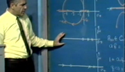
We've seen that behavior in our second-order system. Recall here, we had loop transmission poles at the two X locations. We usually indicate loop transmission poles and zeroes for reference points in our root locus diagram. And recall that the closed-loop pole started at this location for vanishingly small values of A-naught, F-naught. And then, as A-naught, F-naught got very large, why the poles went off, as are the branches, the closed-loop poles left the s-plane as shown.

Well our statement of rule one says that the branches must terminate at zeroes for very large values of the af product, or of A-naught, F-naught. And here, in fact, we have a second-order loop transmission. In other words, the denominator polynomial is second-order in s.

And that function goes to zero. Or the loop transmission goes to zero for very large values of s. And in fact, it goes to zero for large values of s as s squared. In other words, our loop transmission, in addition to having two poles at s equals minus 1 over tau a and s equals minus 1 over tau b, has two zeroes at infinity.

And so, in this case, the branches leave the s-plane. We can consider that as really terminating on zeroes of the loop transmission, which happened to be located at infinity. One of the rules that we'll get later on effectively tells us what direction is infinity for a specific loop transmission. That's another important point.

Rule two deals with the behavior on the real axis. And what I've shown here is an s-plane diagram. Suppose we're concerned with the portions of the real axis where branches of the root locus diagram can exist and, in fact, must exist.

Suppose we'd like to test some part of the real axis, possibly here, to see if that's a possible location for a branch of the root locus diagram. We evaluate the angle of the loop transmission or the angle of g of s at that point. And of course, we've assumed that I am showing in the diagram, the poles and the zeroes of g of s. And when I evaluate the angle of this function, I of course draw vectors from the poles and the zeroes to the point in question.

And, let's see, for every real axis pole or zero to my right, I get a net 180 degrees. The angle of a vector from this zero to this point is 180 degrees. Similarly, the angle of a vector from this pole to this point is minus 180 degrees, or the net angle, since that's a denominator term. But every real axis pole or zero to my right contributes a net 180 degrees.

Real axis poles or zeroes to the left of the point in question contribute nothing to the angle. When I draw vector from this pole, for example, to this point, why the angle associated with that vector is zero. Similarly, complex conjugate poles or zeroes have angles which sum to a multiple of 360 degrees.

A given complex conjugate pair has an angle which sums to precisely 360 degrees. Consider the contribution from this complex conjugate zero pair. This angle plus this angle sum to 360 degrees. Well fine, the condition then is simply that, in order to have an odd multiple of 180 degrees, in other words, to have a minus sign associated with g of s, we must have an odd number of poles and zeroes to the right of us on the real axis, since each one of those poles and zeroes contributes a net 180 degrees to the angle of g of s. Consequently, the only way we can have an odd multiple of 180 degrees is to have an odd number of poles and zeroes to our right.

And so, in this particular situation, for this particular pole and zero configuration of g of s, this portion of the real axis will have branches. There are three poles and zeroes to our right. Similarly, this portion will have a branch or branches. There are, again, one, an odd number of zeroes, in this case, to our right.

Rule three deals with the behavior on portions of the real axis where the branches exist. We determined those portions from rule two. And if, in fact, there are portions of the real axis between either two pairs of poles-- we saw an example of that when we were discussing rule two-- or between two zeroes, why there have to be two separate branches in those locations.

In other words, we've said that branches start at poles of the loop transmission. And consequently, if there are two poles and if the real axis between them, as here, has branches on it, there must be two branches. And the only thing that can happen, as A-naught, F-naught increases-- these branches, recall, start at the poles of g of s, or the poles of the loop transmission for small values of A-naught, F-naught-- as we increase A-naught, F-naught, the two branches come together. But they must eventually leave the real axis so that they can reach zero somewhere. And consequently, they must break away from the real axis at some point between the two poles.

Similarly, if there are two zeroes surrounding a portion of the real axis where branches exist, for some value of A-naught, F-naught, the branches must enter the real axis and then head off toward those two zeroes for larger values of A-naught, F-naught. And so there have to be either breakaway points between two pairs of poles where branches exist, or entry points to the real axis between two pairs of zeroes where branches exist. And we can solve for the location of those entry points by considering an equation, dg of s by ds equals zero.

Let me point out that it's not always necessary to solve precisely for such entry or breakaway points. In fact, my own feeling is that a very real benefit of a root locus technique is that it gives us a way to very quickly sketch important features of a loop transmission or of a closed-loop transfer function.

And therefore, very frequently, we're not interested in exact numerical results. We get enough feeling for what's going on by approximate techniques. However, if we are interested in getting precise numerical results, one of the things we might need to know are the breakaway points. We can get that from the equation that I've indicated.

Again, we've seen this behavior in our second-order system. Notice that here we have the two branches coming together. The real axis in this region must contain branches of the root locus diagram, since there's an odd number of poles and zeroes to our right. In particular, there's one pole to our right on the real axis.

The two branches come together. They break away. They breakaway is at right angles.

And that's always the case, breakaway or reentry to the real axis is always at right angles to the axis, although, the branches may curve immediately after leaving the real axis. So the breakaway occurs at right angles. If we went through the g of s that corresponds to this example and solved for breakaway points, we would find that it was, in fact, at the arithmetic mean of the loop transmission pole locations.

Rule four has to do with the average distance of branches from the imaginary axis. And in particular, it tells us that, if the number of poles associated with the loop transmission-- which I'll denote by a capital P, capital P is the number of poles of the loop transmission, capital Z is the number of zeroes associated with the loop transmission-- if the number of poles of the loop transmission exceeds the number of zeroes by two or more, then the average distance of all closed-loop poles from the real axis remains constant.

The proof of this is an algebraic one. I do it in the book. And I won't do it here.

We begin seeing that behavior in our sample second-order system. Here, again, the average distance of the two loop transmission poles from the imaginary axis is the quantity shown. Since our closed-loop poles start for small values of A-naught, F-naught at these two locations, that tells us that, as the branches move, that average has to be maintained. And in fact, what that implies is something that we didn't get readily from the algebraic development we had already performed, although, we could have gotten it.

What it says is that, when we achieved a value of A-naught F-naught that gets us to move a given distance inward from this loop transmission pole, this branch has moved by precisely the same distance inward from this loop transmission pole location. So as these branches move, they have to move symmetrically. We, of course, find out that that condition is maintained as we get to complex conjugate pole pairs because, again, the average distance, this distance plus this distance divided by 2, equals this distance plus this distance divided by 2.

Rule number five basically deals with what direction is infinity as I had mentioned in the discussion of rule number one. In particular, we're interested in the asymptotes that the branches make for large values of A-naught, F-naught. And the way we evaluate that is as follows.

Consider a root locus diagram. And let's suppose we want to evaluate the angle associated with g of s when we're very far from the origin. In other words, let's consider what happens when we're evaluating the angle of g of s somewhere out here.

As we look from our test point back toward the finite s-plane, why all the poles and zeroes associated with g of s make just about the same angle. The vectors to all of those poles make just about the same angle with the real axis. In other words, when we're evaluating the angle way up there, it doesn't matter much which of these poles or zeroes we draw the vector from, the angle is just about the same.

And consequently, the angle of g of s evaluated at a point far from the origin must satisfy the condition such that Z times theta-- theta is the angle, of course, Z is the number of zeroes-- minus P times theta-- P is the number of poles-- must equal an odd multiple of 180 degrees. We can solve that equation to determine theta. And that gives us the asymptotic behavior of the branches far from the origin. If we did that, we'd get that theta has to be equal to an odd multiple of 180 degrees, actually, over Z minus P.

This really is an error, however, because we're going to allow n to take on all possible integral values, both positive and negative. By convention, since most systems have more poles in their loop transmission than zeroes, reflecting the fact that the world is basically low-pass in nature, we choose to write the denominator in a way that it becomes positive. So we write the denominator as P minus Z.

We've already seen that behavior, again, in the one root locus diagram that we've constructed. Here we have two poles, capital P is 2, Z is zero. And so, if we took n equal to zero and solved for the angles of the asymptotes, we'd find out that angle was 180 degrees divided by 2, in other words, plus 90 degrees.

Similarly, when we allowed n to be equal to 1, we'd find that the angle was three times 180 degrees divided by 2 or 270 degrees. So that gets us an asymptote in this direction. Similarly, if we allowed n to take on larger values, we'd just get cyclical values.

We'd repeat the 90 degrees and 270 degrees that we've already seen. So there's no further information gained from that. In this particular system, the branches coincide with the asymptotes as soon as the branches leave the real axis. That isn't always the case, of course.

The second part of rule five really tells us where the asymptotes intersect the real axis. And that intersection, by an algebraic development, simply comes at the sum of the real part of the poles of g of s minus the sum of the real part of the zeroes of g of s, once again, divided by the number of poles minus the number of zeroes associated with the loop transmission.

So this, again, we could check for our particular system. We have simply two poles. So if we add the real parts of the poles, divide by two, we end up with the asymptote intersection being at the average distance of the poles from the imaginary axis, the poles of g of s, from the imaginary axis.

Rule six tells us the angle that a branch makes either leaving a complex conjugate pole for small values of A-naught, F-naught or entering a complex conjugate zero for very large values of A-naught, F-naught-- in other words, if we were interested in how the branches of the root locus diagram eventually reach this zero for very large values of A-naught, F-naught, a branch might come into that point from somewhere in the s-plane for sufficiently large values of A-naught, F-naught.

And if we were interested in this angle, in other words, the angle that that branch had at the time it entered, or for the value of A-naught, F-naught when it enters that zero or reaches that zero, in particular, this angle, why we can determine that angle by simply evaluating the angle from all of the poles of g of s. Taking the sum of 180 degrees plus the angle from all of the poles of g of s to the zero in question minus the angle from all of the other zeroes of g of s to the zero in question. So this is simply a way of satisfying the odd multiple of 180 degrees at a point in the s-plane.

We can do the same thing if we ask, at what angle does a branch depart a complex conjugate pole for small values of A-naught, F-naught? You simply keep track of the arithmetic. You find out that's 180 degrees plus the sum of the angles when we draw vectors from all of the zeroes of the loop transmission to the pole in question, minus the sum of the angles when we draw vectors from all the poles of the loop transmission to the pole in question, and, as I say, proving that relationship simply involves keeping books to ensure that we have a net angle of 180 degrees.

Rule seven is a powerful one which allows us, quite often, to very rapidly sketch certain important features of the closed-loop transfer function. In particular, what it tells us is that we have a system which includes a collection of poles quite near the origin relative to some others. We're able to ignore the remote poles, and in fact remote zeroes, when we're interested in the behavior of the root locus diagram near the origin.

We can see how that works. Suppose there are a collection of poles and zeroes associated with the loop transmission that are somewhere down near the origin. And then there are some additional ones at much higher frequencies or much further from the origin, possibly out here. This very frequently happens when we look at the behavior, for example, of a transistor amplifier an operational amplifier where there are certain poles, possibly those due to collector to base capacitance or intentional capacitors that we've added to the circuit that are relatively low-frequency in nature.

And there may be some zeroes at relatively low-frequencies as well. And then, very frequently, there are other much higher-frequency poles and possibly zeroes typically occurring out at about omega t, the gain bandwidth product for the transistor. And so this sort of a pattern very frequently exists in electronic amplifiers.

Similarly, we can find this sort of thing a mechanical system. There may be certain poles due to the energy storage and lump masses and springs in the system. And then we get into much higher-frequency poles, poles much more remote from the axis, that have to do with things like mechanical resonances in the system. So this kind of a situation exists quite frequently in feedback systems of interest.

Well to see why we might be able to ignore remote poles and zeroes when we look for the branches in the vicinity of the origin, suppose we had found out that this particular point, in fact, satisfied the conditions necessary to be on a branch in the absence of these higher-frequency poles. In other words, when we evaluated the net angle associated with all of these poles and zeroes, we'd find out that the net angle evaluated at this point was an odd multiple of 180 degrees. We now ask, how does that change if we consider the remote poles?

Well we draw some vectors from the remote poles. But the net angular contribution from those remote poles is quite small. This angle is small. And in fact, the complex conjugate pair sum to a very small angle. While one of these angles is quite large, the sum of these two angles is very small.

So the remote poles don't change the net angle g of s very much, evaluated at this point. And we can make up for that very small change by simply relocating our branch a tiny amount, recognizing that moving our test point a very small amount has a tremendous effect on the angles associated with the vectors from these local poles and zeroes. Consequently, the conclusion that the remote poles and zeroes don't really contribute very much to the behavior of the root locus diagram in this vicinity.

Rule eight is simply a restatement of the magnitude condition. In other words, once we've found a point, s1 in the s-plane where the angle condition is satisfied, the value of A-naught, F-naught necessary to get us to that point on the root locus branch is simply equal to the magnitude of 1 over g evaluate at that point.

Well, with that as a statement of the rules that we're going to use to draw root locus diagrams, I'd like to begin to look at some simple pole-zero possibilities for loop transmissions and then see the corresponding root locus diagrams. The simplest possible case is, of course, a first-order system that has one loop transmission pole on the negative real axis.

So here we have one located, let's say, at a point minus 1 over tau a. About the only rule we need here is rule number one. It tells us that the negative real axis to the left of that loop transmission pole is a possible location for our branch of the root locus diagram. And furthermore, there is only one branch associated with the root locus diagram.

And so combining those two facts tells us that the root locus diagram simply starts here for very small values of A-naught, F-naught, ends at a zero at infinity, which happens to, in this case, lie out along the negative real axis, since we have one pole. If we calculate an asymptote, for example, we find that the asymptote lies at minus 180 degrees. So we get the branch traveling out the negative real axis like so for increasing A-naught, F-naught.

I think it's worth pointing out how that corresponds with an earlier development that we've done. We looked at the single-pole case when we started our discussion of the dynamics of feedback systems. And in fact, under those conditions, we started with an a of s that was equal to A-naught over a single pole, a single real axis pole. And we assumed that F was frequency independent and equal to F-naught.

When we calculated the closed-loop transfer function, we determined that capital A of s was simply equal to 1 over F-naught times 1 over tau as divided by A-naught, F-naught plus 1 over A-naught, F-naught plus 1. Certainly, as we increase the A-naught, F-naught product, the condition under which we construct our root locus diagram, the single closed-loop pole simply moves toward higher frequencies. In other words, the coefficient associated with the s-term becomes smaller and smaller and smaller in the denominator. So we get the behavior that we've indicated.

The second-order case we've looked at in considerable detail. And so I won't look at that again. A somewhat more interesting behavior exists when we consider a third-order system. In other words, a loop transmission that has three real axis poles associated with it.

Our rule number one tells us that this region of the real axis where we have one pole to the right contains branches, and that this portion of the real axis includes a branch. Furthermore, we find that there has to be a breakaway point in this region, since here we have a branch or a pair of branches existing between two poles on the real axis. So there has to be a breakaway somewhere between them.

We'd actually expect, let's see, that that breakaway would have to be a little bit to the right of the midpoint, if we keep track of the average distance, because we recognize that this branch is continuously moving to the left. Consequently, we'd anticipate that the breakaway would have to be just a little bit to the right of the midpoint here in order to keep the average distance from the imaginary axis a constant. So we might get a breakaway somewhere in here.

We also can calculate the angles of the asymptotes, which is useful in this case. We have three poles and no zeroes. And consequently, we would expect asymptotes at plus 60 degrees, 180 degrees divided by 3, at 180 degrees, which is 540 degrees divided by 3.

And, let's see, we'd also expect another asymptote at 270 degrees for this particular system-- I'm sorry, at 300 degrees at minus 60 degrees, that's 900 degrees divided by 3. So we'd anticipate, for large values of A-naught, F-naught, that there would be asymptotes at plus and minus 60 degrees and at minus 180 degrees. And the asymptotes intersect somewhere on the negative part of the s-plane, since the real parts of all of these poles are negative.

And putting those things together, we'd conclude that the behavior might be something as follows. These branches eventually getting into the right-half plane, implying, of course, this third-order system can become unstable for sufficiently large values of A-naught, F-naught. And ultimately, we get asymptotes of plus or minus 60 degrees associated with that complex conjugate pair of branches.

It's interesting to point out a special case that we've investigated earlier of this three-pole situation, in particular, one where we have three coincident poles. If you recall, we looked at this situation when we discussed the possibility for instability in feedback systems. And in that case, the root locus diagram was somewhat degenerate.

And, in fact, the branches immediately parallel the asymptotes, or lie along the asymptotes, look like this. And, in fact, if we keep track of the arithmetic involved, if this is 60 degrees and this point is minus 1 over tau, then this branch crosses into the right-half plane at s equals plus j radical 3 over tau, since this angle is 60 degrees. We can also use, as an aide to constructing more accurate root locus diagrams, if we feel the need to do that, some rather simple arithmetic calculations. And I'd like to illustrate that in closing.

Let's consider an a of s f of s that includes three poles. In particular, we have A-naught, F-naught over three real axis poles. One located with a time constant of 1 second, in other words, at s equals minus one. Another one located with a time constant of a half a second at s equals minus 2. And finally, the third real axis pole with a time constant of 1/10 of a second located at s equals minus 10.

And I have that one done fairly accurately here. In other words, we show the loop transmission pole locations at s equals minus 1, s equals minus 2 and s equals minus 10. We've already looked at some of the features of this sort of a diagram. In particular, branches exist between these two poles and to the left of the third loop transmission pole. The asymptotes are at plus and minus 60 degrees and at 180 degrees.

For this particular case, the asymptotes intersect the real axis at minus 1, minus 2, that gives us minus 3, and another minus 10, in other words, minus 13 divided by the number of poles, which is three. So the asymptotes intersect the real axis at minus 4 in the third. And using that information, we can begin to sketch the behavior of our root locus diagram.

Note that, if we totally ignored the third pole-- we have this rule that says we can ignore remote poles and zeroes when we're interested in the behavior near the origin-- if we totally ignore the third pole, we'd anticipate the breakaway would occur at the arithmetic mean of the location of these two loop transmission poles. That's what happens in only the two-pole case. That would tell us the breakaway would occur at minus 1.5 on the negative real axis.

If we actually do an exact calculation of the breakaway point, we find that it really occurs at minus 1.47. So in this particular system, where we have two poles located within a distance of two units of the origin, a third pole located 10 units from the origin, we find out that we could predict breakaway very accurately, totally ignoring the third pole. We can get some other important features of the diagram, if we're interested in that, by using rather simple numerical techniques. For example, we talked about the Routh criterion last time. And we found that that was a rather simple numerical method that will allow us to determine the number of closed-loop poles of the transfer function in the right-half plane.

Another way to use that-- as I indicate in the book and I believe you tried with some of the homework problems last time-- is to determine, for example, what value of A-naught, F-naught will result in a complex conjugate pair of poles lying on the imaginary axis. If we do that development, we can determine the value of A-naught, F-naught, which gets the closed-loop poles to these two points. And furthermore, we can also determine the imaginary component when the poles cross into the right-half plane. And if we perform that calculation, we find that these branches cross into the right-half plane at points plus and minus j 5.65.

Furthermore, the value of A-naught, F-naught necessary to get a pair a complex conjugate poles in the right-half plane, in other words, to make this third-order system unstable, is an A-naught F-naught value of 19.8. We can also use rather simple algebraic manipulations to determine other important features of the diagram or as a design aid. For example, we recognize that we have one degree of freedom in this particular development.

The only thing we're able to control is the A-naught, F-naught product. We're constructing the root locus diagram as a function of A-naught, F-naught. And that's the single degree of freedom that we have.

So we expect that we'd be able to control one feature of the closed-loop response. For example, we might choose to fix the location of the real axis closed-loop pole. That's not a particularly useful constraint, but it's at least one possibility.

Another one which is probably a more useful constraint might be to exercise our one degree of freedom in order to set the damping ratio of the complex conjugate pole pair. In other words, we recognize that, as we increase A-naught, F-naught, our closed-loop poles move along these branches. And suppose that I would like to design for a given damping ratio associated with the closed-loop pole pair-- this closed-loop pole pair certainly dominates performance since it's the pole pair closest to the origin and much closer than the third pole.

Well what we can do is write the polynomial, the characteristic equation of the closed-loop transfer function. And if, for example, we'd like to set up for a damping ratio of 0.5, in other words, these branches, 60 degrees from the real axis, that implies a given relationship among the coefficients of the characteristic equation. And we can use rather simple algebraic manipulations to determine the value of A-naught, F-naught that matches those conditions.

I do that in the book. When we go through that development, we find out that this system has a closed-loop damping ratio for the dominant pole pair of 0.5 for an A-naught, F-naught of only 2.2. So in this particular system, we find out that, if we'd like to maintain a reasonable amount of damping where a reasonable amount of damping might be a damping ratio for the dominant pole pair of greater than the 0.5., we can only achieve an A-naught, F-naught product of 2.2, or a desensitivity by our original definition of 3.2.

Next time, we'll look, from a root locus point of view, at how we might be able to improve that situation. What should we do to certain kinds of feedback systems in order to increase the desensitivity we can obtain before we reach a given degree of instability? Thank you.