James K. Roberge: 6.302 Lecture 01
[MUSIC PLAYING]
JAMES K. ROBERGE: Hi, I'm Jim Roberge, and I'm with the Department of Electrical Engineering and Computer Science at MIT. I'd like to welcome you to our subject on feedback systems. The material we'll be covering is in the field known as classical feedback techniques. And I'd like to point out that there's a very real difference between this category of material, classical feedback techniques, and what's now known as modern control techniques.
There's another subject in this series, one given by Professor Athens, also here at MIT, that covers one aspect of modern control. But we won't be looking into those sorts of things.
I think one of the fundamental differences between classical control and modern control theory is that an underlying assumption in many of the ideas in modern control is that you're able to make decisions on a time scale very fast compared to the dynamics of the systems involved. You're then able to do optimization. A lot of the techniques in modern control theory come from the calculus of variations. And what you're able to do is really explore the effects of a given strategy for control in a short period of time compared to the dynamics of the system before the system changes very much.
This kind of an approach is very good if, for example, you have a satellite in orbit around the earth and you'd like to figure out, what's the optimal trajectory to get to the moon, a minimum fuel trajectory, or something like that. Because you recognize that that trip is going to take you several days. And yet, we currently have the ability to do calculations of simulations of that sort of dynamic system in a very, very short period of time. And so we can investigate and detail the effects of various control strategies.
However, if we look at another kind of system of interest. For example, a high-speed amplifier. Suppose we're worrying about a 100 megahertz type of operational amplifier. We're really not able to make decisions on a time scale fast compared to the dynamics of that system for basically fundamental reasons.
If we had devices that allowed us to make decisions on that sort of a rapid time scale, why what we'd do is redesign our amplifier to use those devices, and thereby increase the speed of the amplifier. So in certain applications, in a very large class of important applications, we find that this disparity between the dynamics of the system and the speed with which we can make decisions doesn't exist and we're forced to use other control techniques. We'll be looking at those kinds of classical control techniques, or what we might call ancient control theory.
This material has been available for a period of time. In fact, I think the pioneering work in classical control theory was done starting during the second World War, principally at Bell Laboratories and here at MIT in the Radiation Laboratory. And we'll be basically reviewing some of that material and seeing how it applies to a collection of modern systems.
One of the themes throughout this subject will be the application of the techniques we're discussing to real world kinds of systems. I think there's a tendency to feel what the techniques we have are very special purpose, very dedicated to single kinds of applications. But we'll see that's just not true. We'll develop analytic and design techniques, and then we'll illustrate those analytic and design techniques by applying them to a very wide range of systems. We'll look at purely electronic systems. Operational amplifiers, for example, and we'll see how we apply the techniques we've developed to those kinds of circuits. We'll look at some examples of mechanical systems, [UNINTELLIGIBLE] mechanisms or systems where at least one of the variables is a mechanical one. And we'll look at how we apply some of these ideas to certain kinds of [UNINTELLIGIBLE] mechanisms. So we'll see a variety of applications for the techniques that we'll develop. And we'll illustrate many of these applications with actual operating systems. We'll see a number of examples of that sort of thing.
I'd like to indicate some of the additional material that we'll have for the course besides the videotape material. The book that we'll use is this one. It's called Operational Amplifiers: Theory and Practice. But that's really somewhat of a misnomer. This is basically a collection of things that I had wanted to write for quite a while. And a large part of the text does really deal with classical feedback. In particular, we'll be concentrating on the materials in chapters one through six in the book. The material in chapter 13 gets back to classical feedback concepts and we'll look at that in detail. And then we'll use certain examples from chapters 11 and 12 out of this book. So we'll cover about half the material in the book as we go through the subject.
We will also have problems in the subject that are basically taken from the book, in most cases. And so the book is very, very closely linked to the subject. This book and the subject for that matter, are ones used here at MIT in a subject called 6.302, which is again entitled Feedback Systems. And the material I'll be presenting has been abstracted from that subject for use here.
In addition to the text, we'll have a study guide. The study guide will include the visuals that we used here, the blackboard material as well as the view graphs that we use. The study guide will list the problems that will be assigned in conjunction with the various lectures. And we'll also have solutions to problems included in the study guide.
I'd like to spend just a moment talking about the prerequisites I anticipate for participation in the subject. We'd like you to have a reasonable background in linear system manipulations. Basically, at an s-plane level. You should be familiar with the usual kinds of s-plane manipulations. How do you find the magnitude in phase for purely sinusoidal excitation? For example, if you're given a pole 0 plot for a system transfer function, that sort of thing. So we'd like to have a reasonably good appreciation of linear system concepts. But we won't really depend particularly heavily on using a big sledgehammer of Laplace to attack the systems. We'll spend very little time actually doing things like partial fraction expansions in order to take inverse transforms and that sort of thing.
So while you do have to have an appreciation of transfer functions of the significance of various pole 0 configurations and that sort of thing, we really won't be spending very much time looking at the formal mathematics of Laplace kinds of manipulations.
Also, really because we use them so frequently for examples, you should be able to look at an operational amplifier connection and decide that if the amplifier had ideal characteristics-- the usual kinds of things that we list in connection with an operational amplifier-- very high open loop gain, very high input impedance, very low output impedance, the usual kinds of good things that we talk about in connection with operational amplifiers. Given those constraints, that the amplifier is effectively ideal, you ought to be able to predict what the ideal closed loop gain should be by looking at the topology for a least relatively straightforward operational amplifier configurations.
Again, that's a talent that I think most of you have. Operational amplifiers are so all-pervasive at present that most people have picked up the facility to look at a connection and see what the objective of the connection is. If you have any concerns about that, I go through those kinds of calculations in chapter one, and I encourage you to review the material there in order to gain that degree of facility.
Well, what do we mean by a feedback system since that's what we're going to be studying throughout this subject? I think a feedback system is one where we attempt to control an output variable in response to a command. But the important distinction in a feedback system is that at least part of the information used to control the output variable, itself, is derived from measurements that we make on the output variable. So this idea of looking at the variable that we're trying to control and using that information, at least in part to control the variable itself, is central to the idea of feedback systems.
There's certainly many examples of those that we're all familiar with. We can look at most electronic amplifiers, audio amplifiers, for example in entertainment systems, include feedback. It's very difficult to get the kinds of characteristics we'd like to have in a good quality audio amplifier without using feedback. We've certainly all seen numerous examples of mechanical systems. Ways, for example, of moving aircraft control surfaces in response to commands from the cockpit. Ways of pointing radar antenna, again, in response to commands generated elsewhere. So we've seen examples of mechanical systems of that kind.
There's also a very important class of feedback system known as a regulator, and we're familiar with examples of those. A home heating system where you measure the temperature of a room and control the furnace in order to maintain that room temperature at some set point value. Similarly, the system involving the iris that regulates the amount of light that strikes your retina. Here again, it's a feedback system. Somehow you measure the total light flux striking your retina and the iris reacts in a way to regulate that total amount of light flux that hits the retina. So here's a biological example of a feedback system.
Interestingly enough, you can make measurements on that system by appropriately stimulating it. You can get the same sorts of instabilities that we oftentimes see in man-made control systems.
I'd like to show some elements that are common to many of the kinds of feedback systems that we're going to examine. Here we have a sort of diagrammatic representation of a feedback system. We have an input variable and, of course, an output variable. And the objective is certainly to make the output variable bear some known relationship to the input applied to the system.
And the way we accomplish that is by measuring the output. Obtaining some measure of what the output's value is, or certain characteristics of the output. We do that with a measuring or a feedback element. And what we do is compare our measure of the output variable with the applied input variable. So we have some sort of a comparator that develops an error. The error being the difference between the input or the command variable and our measure of the output variable.
We then amplify that error signal, and change the output. Drive the output as a function of the amplified error signal. And of course, the objective is to drive the output variable in such a direction to reduce the error signal. To make the measured function of the output variable be in better agreement with our input. So the system works to drive the output in such a way that the error tends towards 0.
And that's, at times, complicated by disturbances that may be applied to the system at some point. I happen to have shown the disturbances here in conjunction with the amplifying element, but that's not necessary. The important point is that our attempts to make the output, or the measure the output correspond to the input, may be complicated by disturbances that are applied to the system.
I think we can look at a fairly familiar example and see how it corresponds to that sort of diagrammatic representation of a typical feedback system.
Here we have a rather familiar operational amplifier connection. This is called a non-inverting amplifier connection. We have an input voltage, V sub i, which I apply to the non-inverting input terminal of our operational amplifier. The quantity, a, is the open loop gain or the open loop transfer function of the operational amplifier. And we then get an output from our operational amplifier. That output is attenuated by a network involving the resistors R1 and R2. And the voltage at the output of that network, we'll call V sub f. That's actually the voltage fed back in this particular system.
We also then get an error, which is really the difference between the input voltage, Vi, and our measure of the output. Here we have the output voltage. Our measure of the output involves, in this case, simply the attenuation ratio of the R1, R2 network. That assumes the amplifier is ideal in the sense that it doesn't load this network.
We generate an error voltage proportional to the difference between the input and the fed back voltage. So we see aside from the disturbance that I indicated is a possibility in our diagrammatic feedback system, here we have the elements central to a feedback system-- an input, an output, a measure of the output, an error that's the difference between the input and that measure of the output. And then, the amplifying element that amplifies the error signal and drives the output accordingly.
I'd like to indicate a notation that I'll use throughout the subject. And what we will do is the following. We use a combination of a variable and its subscript to indicate the class of variable that we're dealing with this. And this will become important later on as we look at a wider variety of systems. But the notation is as follows.
If we use a lowercase variable and a capital subscript, we're talking about a total variable or time variable. In many cases, we'll be linearizing as one technique for analyzing systems. And when we do that, we very frequently find it convenient to decompose a total variable into a sum of an operating point variable and an incremental component about that operating point.
The way we designate an operating point is capital V sub capital I. We use capitals on both the variable and the subscript.
We'll designate the incremental component about that operating point by a lowercase variable and a lowercase subscript.
And the final permutation of the capital variable and the lowercase subscript, we'll use for a frequency domain representation. A complex amplitude or a Laplace transform, that sort of thing. And you notice that's the notation I've used here. That allows us the possibility of talking about a transfer function for the amplifier. We'll see very rapidly-- not actually in this session, but very shortly we'll see that we'll begin to worry about how these systems behave when the quantity a is frequency dependent. By using the complex amplitude of the frequency domain notation we allow ourselves that capability.
Well, let's go ahead and develop the closed loop gain for this very simple non-inverting operational amplifier configuration.
The amplifier, of course, provides an output V out, that's equal to it's open loop gain or open loop transfer function times the differential voltage applied to the operational amplifier. So the output voltage is simply a times the differential input voltage. That voltage is Ve in our schematic diagram. And the voltage Ve is simply equal to the difference between the input voltage applied to the overall system, Vi and our measure in the output, V sub f.
V sub f, in turn, is the attenuated version of the output. In this particular system, R1 over R1 plus R2 times V out. Again, this presupposes that there's no loading at the input in the amplifier, so that the attenuating network, the R1, R2 network isn't affected because of input impedance associated with the operational amplifier. We're able to write the voltage, Vf, as simply being equal to R1 over R1 plus R2 times V out.
I'd like to introduce a notation again, that we'll use almost universally throughout the subject. Let's call this fraction f. In general, the relationship between the output variable and the quantity that we feed back in our feedback system is f times V out. The fed back quantity is f, the feedback function, times V out. Again, I emphasize the fact that this expression is true only in the case where we can ignore loading in the operational amplifier at the input of the operational amplifier. We could certainly get some modified f, some different value for f, if we did have to worry about loading.
We can then combine these equations and conclude that V out is equal to a times Vi minus f V out, simply combining these equations. And that allows us to write the closed loop transfer function V out over Vi. And we use that expression often enough so that I'd like to introduce, again, a standard notation that we'll use for the closed loop gain or the closed loop transfer function of our operational amplifier. It, at times, will be a function of s, the complex variable s. But anyway, our closed loop transfer function will be capital A, and that's equal to little a-- in this case, the open loop transfer function, or the open loop gain of the operational amplifier-- over 1 plus af. That's simply the result of combining this set of equations.
We'll frequently find that it's convenient to indicate the relationships that exist in a feedback system in terms of a pictorial representation. And that sort of pictorial representation is known as a block diagram.
And I have an example here of a block diagram. The reason that we do this is not because it gives us any information that we didn't have before. In fact, we can certainly construct a block diagram by looking at the equations that describe the behavior of the system. We can go back and forth readily between those quantities. But oftentimes, the topology that we see when we get a block diagram or when we develop a block diagram, gives us a very nice feeling for the way signals are interacting in a feedback system. And so I think the advantage is that kind of insight that the pictorial representation very frequently gives us.
And here's an example of a simple block diagram. In fact, one for the system we've just described. There are three kinds of elements, if you will, in a block diagram. There are lines, and lines represent variables in our block diagram. For example, this line represents the output, V out. This point in the block diagram is equal to the difference between V out times f And Vi. And that's simply equal to the quantity Ve, which we mentioned earlier. So a line represents a variable.
We have blocks, and blocks simply scale variables. Here we have V out going into a block that provides a gain of f. And the output of that block is then the quantity V sub f that we mentioned earlier.
We also have a third kind of element, a summing point where we algebraically combine variables. Here we have Vi and Vf. We get the output of our summing point as being equal to the difference between Vi and Vf. Vi minus Vf, and that's Ve. So here we have a pictorial way of representing our system.
The closed loop transfer function for this configuration then, we can get the following way. We've already derived this expression by going through the algebraic manipulation. And we can also get that pictorially. We may find out that what we do is develop a block diagram by a series of manipulations that reduce a more complicated block diagram. There's examples of that in the text. And in fact, some of the homework problems associated with this session will have you go through some block diagram manipulations. But we may find out that for a more complicated system, we start with a more general block diagram, one that has possibly multiple loops or something. But we're always able to go through a series of manipulations at least for linear systems until we finally get our block diagram down to this form.
Here it came out directly, we notice as a very nice 1:1 correspondence between that block diagram and the actual system that we started with. We have the input. We have Vf. We have f times V out all appearing in the block diagram. The function of the summing point in the block diagram is performed, of course, by the differential input on the operational amplifier here. So here there's a very, very nice 1:1 correspondence between the physical system and the block diagram. That almost perfect match doesn't always exist, but frequently does.
In any case, we can, by using block diagram manipulations that we'll look at, reduce a complicated system generally to this sort of configuration where we have an input, a single path between the input and the output, and we'll try to stick with the notation where we use a lowercase a for that path. And then a single feedback path from the output back to the summing point. And we'll try to use the notation f pretty much generally for that feedback path or feedback transfer function.
When we've reduced the system to this configuration it, of course, obeys exactly the equations that we've written down here. And so we can, by inspection, write the closed loop gain. We can recognize that the ratio-- the relationship between the output and the input, V out over Vi, which is by definition capital A, the closed loop gain of the system, is always equal to the forward path a over 1 plus af. If we have this standard form of forward path a, a feedback path f, and an inversion associated with the feedback path that's shown here at the summing point.
The quantity af that appears in this expression is a very important one for feedback systems. And as we'll see, that quantity, the af product, controls many of the important parameters that we associate with the feedback system. And in fact, it has a name. We call the loop transmission for a feedback system in this standard form of the quantity minus af is loop transmission. Loop transmission has a very, very nice physical significance. Let's go into our system, either on a block diagram level or the actual physical system. And what we can do is break the loop. Actually, we break the loop at any point.
Let's say here. And we suppress all input. So we'd set Vi to 0. And then we test the system by applying a test generator. Let's put one in here. And we observe the signal that the loop returns in response to a test signal.
Well, let's look at the signal Vo, that's the signal that comes back at the point where we had opened the loop or broken the loop. And the relationship between V out and Vt is simply f times minus-- we get an inversion associated with the summing point. So we have f times minus 1 times a, or minus af for the single returned by the loop when we test it. Minus af is the loop transmission of this system.
We can do that very easily on a block diagram basis. We can do the same thing in our physical system. There may be a practical problem associated with breaking the loop. But there may be the amplifier may saturate or something like that. But at least if we ignore that for a moment conceptually, we can determine the loop transmission by exactly the same kind of manipulation.
We break the loop. Possibly here is a good place. We suppress the input source. Make that voltage source 0. Apply a test signal. And again, find out that when we observe the signal that comes back in response to a test, why we get the test signal times an attenuation ratio, R1 over R1 plus R2. We get an inversion because the signal happens to go in to the inverting input of our operational amplifier. And then the signal returned is a times f times the inversion minus af.
Providing a and f both have the same sign, the polarity, or the sign associated with the loop transmission, is negative. And so this is an example of a negative feedback system. And in general, those will be the kinds we're studying. We could also look at positive feedback systems. We'll see an occasional example of a positive feedback system. But generally, for our purposes, they're not quite as useful. And so we'll focus our attention principally on negative feedback systems.
If we're concerned about whether a system is a negative feedback system or not, there's a fairly nice test. We could, for example, start with a system, start with a value of f equal to 0, and then let f go toward the value that it actually has in the system. If under those conditions the magnitude of the closed loop gain, the magnitude of capital A decreases as we increase f from 0 toward its actual value, we have a negative feedback system. And so that's an easy way to test to see if a feedback system is, in fact, a negative feedback system.
Well, why do we do this? What's our interest in building feedback systems? Let's again, look at our closed loop gain expression. The part that's valuable to us is the following.
Suppose we have a sufficiently large af product. Suppose the magnitude of af is much, much larger than 1. Well, then our closed loop gain expression-- in evaluating the closed loop gain expression, we're able to ignore the 1 in the denominator compared to the af product. And consequently, the denominator is approximately equal to af. As a result, capital A is simply approximately equal to 1/f. That's the feature that we're really looking for. And the reason is as follows.
The quantity a, which is the forward path of our feedback system, very frequently isn't particularly well known. Usually the gain, the active elements in our feedback system, are concentrated in the forward path. And as a result because of uncertainties associated with the active elements, possibly temperature or time dependencies associated with air characteristics, this quantity may not be particularly well known.
Conversely, we very frequently find that it's possible to mechanize the function f, the feedback transfer function, by means of stable passive components. In our particular example, we used a resistive attenuator in order to mechanize the feedback element.
Well, we can buy passive components. We can buy resistors with ratios that are known to almost any degree of precision we want. If we go to a resistor manufacturer with a large enough of gold, they'll give us resistors whose ratio can be controlled to a part in a million if we care to do that. It's very, very difficult, in fact, impossible to build an amplifier not using feedback techniques where the gain of the amplifier itself is controlled to a part in a million. We just find out that that's not a possible thing to do no matter how much money you have.
So what we do by using feedback, is find a way to make the closed loop gain, the gain with feedback dependent on a quantity that we may be able to define very precisely, or specify very precisely. And we make ourselves largely insensitive to variations in a subject only to the constraint that a is big enough, so that the af product is large compared to 1. If we're able to do that, if we're able to say well a is big enough, then in fact we can make-- or the forward path a, little a, is large enough. We're able to make the closed loop gain dependent on the well known characteristics of the feedback element.
We can emphasize that concept by calculating the change that occurs in closed loop gain as a function of changes in open loop gain. And again, we start with our forward path transmission. We start with our expression for the closed loop gain capital a being equal to the forward path over 1 minus the loop transmission. And if we differentiate this expression, we get that dA is equal to da, little da, over 1 plus af squared.
Well, we're not interested really in relationships between absolute changes in the forward path gain and the closed loop gain. But rather, in the relationship between fractional changes in the forward path gain and in the closed loop gain. So what we'll do is divide this expression. We'll divide the left side by capital A. We'll divide the right side by the equivalence for capital A, little a over 1 plus af. When we do that we find out that the fractional change in closed loop gain, dA over cap A, is equal to the fractional change in forward path gain, little da over little a, times an attenuation factor 1 over 1 plus af. This quantity we'll call the desensitivity. And what it does is indicate how our feedback topology desensitizes the closed loop gain to changes in the forward path gain.
This again, is a very important quantity. Clearly, we're interested in having systems that have large desensitivity so that we can tolerate large changes in the forward path gain and get minimal changes in the closed loop gain of the system. One of our design objectives very frequently will be to build systems that have large values for desensitivity.
Notice that the desensitivity is obtained really, only in exchange for starting with a greater amount of forward path gain than we actually need. We're designing a system that has a final closed loop gain that's a over 1 plus af. Capital A is little a over 1 plus af. However, we start with a forward path gain of little a. So our feedback topology attenuates the gain below that which we started with by a factor of 1 plus af. And that's precisely the amount of desensitivity we get. So we get desensitivity only in exchange for starting with a forward path gain that's larger than we actually need. So that's the price we have to pay in order to achieve the desensitivity we're interested in.
I think the ability to automatically desensitize a system to changes in forward path gain is the only property that's really intrinsic to a feedback topology. I think there's a tendency on the part of people when they begin to worry about feedback systems to associate almost magical properties with them. And that's just not true. Feedback generally doesn't allow you to do many of the things that you can't do without feedback.
For example, feedback never gives you a mechanism for detecting signals that you couldn't detect by other methods. Certain detection schemes may be more conveniently realized as feedback topologies, but we can't use feedback as some sort of salvation to rescue signals from noise that we couldn't do otherwise. There's a whole collection of those sorts of things that at first there's a hope that feedback might help with. In reality, feedback doesn't offer that sort of panacea.
The only thing it does do-- I believe the only fundamental property of feedback-- is that it gives us desensitivity in exchange for excess forward path gain.
One of the other features of feedback systems, another feature, is that feedback systems frequently give us ways of modifying input and output impedances associated with systems. Either mechanical impedances. For example, compliances or stiffnesses in mechanical systems, or the equivalent electrical input and output impedances. And I'd like to look at that for a moment.
Here we have, again, a familiar operational amplifier configuration, an input. I've indicated the operational amplifier now as a dependent generator whose magnitude is a times the error voltage, and then some output resistance, r out, the output voltage. And I feed that back to the inverting input terminal of the operational amplifier, so this is a familiar follower connection.
I've also indicated a test source that can apply disturbance. In this case, a disturbing current. And what I'll do is use that disturbing current to test the output impedance or output resistance of our configuration. So what we'll do is effectively measure the output resistance of this configuration by determining the relationship between changes in output voltage and changes in this disturbing current. That's, of course, by definition the output resistance of our configuration.
Well, first, let's make a block diagram for this system. We do that. We have our input voltage. We get an error that, in this case, is the difference between the output voltage and the input voltage since we have a direct feedback connection in our system. In other words, we have an f of 1 for this particular system. Remember, there's a wire directly back from the output to the inverting input.
We get an error voltage that's the difference between those two quantities. The dependent generator associated with the operational amplifier provides an output voltage that's a times the error voltage. But there's another term besides the output voltage of the dependent generator associated with V out. In particular, the drop across this resistance R out, the output resistance associated with the operational amplifier. And since the input current to the amplifier is assumed to be 0, the disturbing current Id, all flows through the output resistance of the amplifier. And we can model that in our block diagram form by taking Id, scaling it by the output resistance. This variable is then the voltage across the output resistance, r0. We add that voltage to the voltage from the dependent generator to get the actual output voltage in the amplifier, and we feed that back.
Well, here's a system that has actually, a desired input, and then a disturbance. And we can write the output for our system as the superposition of the responses to the desired input and the response to the disturbing current.
If we do that, we get the output. And now let's do the component dependent on the input voltage. When we have our standard feedback topology, a forward path, a feedback path, the result is always the same. The expression is always the same. It's the forward path over 1 minus the loop transmission. So let's see. The forward path is a, the loop transmission is minus a. There's nothing else in the loop, so the relationship between V out and Vi is the forward path a over 1 minus the loop transmission 1 plus a. V out is a over 1 plus a times Vi. And now we have another component. That component being proportional to Id.
Well, there's a scaled factor before we even get in to the loop associated with Id. That scale factor is r0. We can drag it out in front in our expression. And then we can calculate the transfer function or the gain from this point to the output. The forward path for that transfer function or that gain is simply 1. And again, the loop transmission doesn't change. The loop transmission for a feedback system is an intrinsic property, a fundamental property of the system. It has nothing to do with what we consider the input and the output of the system. And so we get the same denominator expression, 1 plus a or 1 minus the loop transmission. We get r0 times 1 over 1 plus a. And that's the scale factor that links output voltage to disturbing current.
And what we see is that fine, we get an output voltage that's very nearly equal to the input voltage. At least in the case where a is very large. We get an output resistance, the ratio between changes in output voltage and disturbing currents, that's simply equal to the open loop output resistance. The resistance that the amplifier would display in the absence of feedback divided by a very familiar expression, 1 minus the loop transmission. We get r out, the open loop output resistance, over 1 minus the loop transmission for the output resistance with feedback.
Here, in contrast to the desensitivity issue, we're able to accomplish this sort of thing at least conceptually, without feedback. Consider the following.
Let's take exactly the same amplifier. In other words, an amplifier that has this model. We have a dependent generator in here whose magnitude is a times the voltage applied to the amplifier. And then, let me in a very brute force way load the amplifier with a resistor whose value is r out divided by a. In that case, we would find-- let's see. When we went to calculate the gain from here to here, V out over Vi, we'd get the gain associated with the dependent generator, which is a. And now we'd get an attenuation ratio that's dependent on r0 over a and the output resistance of the amplifier. That's our attenuation ratio. We have an external resistor r0 over a. There's an internal resistor that's r0. And so we get an attenuation ratio r0 over a divided by r0 plus r0 over a.
And if we can simplify this expression a bit, we find that the gain for this expression, for this configuration-- exactly as it was up here, the relationship between output voltage and input voltage-- is simply a over 1 plus a.
Similarly, if we calculated the output resistance of this configuration, it would be r out over a in parallel with r out. And if we simplify that, we'd find out it was r out over 1 plus a. So here conceptually, is a topology that gives us both the same voltage gain and the same output resistance as the feedback topology.
This isn't to imply that this is a good solution. In fact, I think we appreciate that loading an operational amplifier with a resistor whose magnitude is its output resistance, which may be ohms, divided by its open loop gain, which may be hundreds of thousands, is probably quite an impractical thing to do. But at least conceptually, at least on a block diagram or a mathematical level, we're able to get the same performance with a topology that doesn't include feedback. We don't do any worse with a feedback solution, but we don't do any better in terms of scaling impedances and so forth.
I went through this sort of a discussion one time when I presented this material at MIT, and a student of mine who was a very gifted student. And in fact, was kind enough to do some reviewing of my book in note form, came up to me after the lecture and said, Jim, you really give aid and comfort to the enemies of feedback by that kind of presentation. He said, I think a better way to look at it is the what you do is you build a feedback system really to take advantage of its fundamental property, the desensitivity, and you find out that you get a whole lot of other things to go along with it. For example, it gives you a way of scaling impedances.
We'll see you next time it gives us a way of dealing with certain kinds of noise in a convenient method. It doesn't give us a way of emanating noise. It doesn't give us a way of improving signal to noise ratio beyond what we could do with an open loop solution. But it gives us a very convenient way to handle certain kinds of noises. And I think that's a good way to look at it. We build a feedback system for its fundamental advantage. That of desensitivity. We happen to get a lot of other things thrown in for free.
Returning for a moment to the issue of impedances. A number of people make a big, big issue about topologies involved with impedance modification. And they talk about shunt feedback, and series feedback, and all those kinds of things. And I just happen not to believe that. Or not to believe that's the right approach. I think that feedback is feedback. And the way that impedance scaling occurs is very, very easy. Or it's easy to see.
What happens is that feedback scales the impedance level of a system, either in its output or its input. And the scaling factor is always the same. It's always 1 minus the loop transmission.
Now, does it lower the impedance, or does it raise the impedance? Well, all we have to do is look at the topology. We don't have to assign names with to this and so forth.
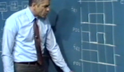
Here we have a topology where we're bringing back the output. We're applying our input signal in a location where the input impedance should be very, very high. We'd find out that if we looked at this configuration, we would get a very high input impedance. We'd scale the input impedance in the absence of feedback by a factor of 1 minus loop transmission. We'd up it. But we're bringing back information about the output voltage. The implication being we're trying to hold the output voltage fixed. In order to do that, we need a low output impedance. Or that's what we're trying to accomplish. and so, when we look to the output impedance, we find that it's the output impedance in the absence of feedback this time divided by 1 minus the loop transmission.
Let's look at another topology. Let's ask, what impedance do we see at this point? Well, what are we doing here?
Here we have a configuration where we ground one input terminal to the operational amplifier. We apply our test signal to the other point. But notice, of course, that the feedback in the system should fight to keep the voltage between these two terminals very small. We have a very high gain operational amplifier. That should show up as having a very small input resistance. We can see how that happens.
Let's apply a test voltage in order to really determine the input resistance. If we apply a test voltage generator, measure the result in input current, the ratio of those two is simply equal to the input resistance.
If I apply a test voltage Vi over here, the amplifier, assuming its output resistance is 0, gives me a voltage minus a times Vi over here.
Consequently, the current through the resistor, which is equal to the input current, is simply equal to the voltage here minus the voltage here. That quantity is 1 plus a times Vi divided by the resistor value. Current here is this voltage minus that voltage divided by R.
If I take the ratio than, Vi over Ii, which is equal to the input resistance-- this may be a little bit confusing. But R sub i I'm now implying is the input resistance for the configuration. It's simply equal to R divided by 1 plus a. In other words, what we've done is lower the input resistance by a factor of 1 minus the loop transmission, compared to the value that we'd see without feedback. If the amplifier gain were 0, we'd have no feedback. This point would always remain grounded. We'd see an input resistance simply equal to R. Feedback scales that by an amount 1 minus the loop transmission. In this case, it lowers it.
We have a topology where what we're doing is designing for a low impedance at this point. Because of that topology we scale lower the effective resistance by a factor of 1 minus the loop transmission. So we can simply look at the topology, see if we're trying to increase or decrease a resistance or an impedance by virtue of the topology, and the scale factor is always 1 minus the loop transmission.
Next time we'll continue our discussion of the properties of feedback systems. In particular, we'll see how feedback systems do affect the noise associated with a system. We'll also look at how feedback can be used to moderate the effects of certain kinds of nonlinearities in a system. Thank you.